

The Scientific Method in Political Science
These notes are a combination of notes from Matt A and Estelle H. Enjoy.
 Topic One: What is the scientific method?
- Overview
- Science as a body of knowledge versus science as a method of obtaining knowledge
- The defining characteristics of the scientific method
- The scientific method and common sense
The nature of scientific knowledge claims
Four Characteristics of the Scientific Method:
What are the hallmarks of the scientific method?
Empiricism: require systematic observation in order to verify conclusions, tested against our experience
Intersubjectivity require systematic observation in order to verify conclusions, tested against our experience
- Explanation: the goal of the scientific method. Generalized understanding by discovering patterns of internal relationships among phenomena. How variations are related.
- Determinism: a working assumption of scientific method. Assumption that behaviour has causes, recurring regularities & patterns. Causal influence. Must recognize that this assumption is not always warranted.
- Empiricism requires that every knowledge claim be based upon systematic observation.
Assumptions:
Our senses (what we can actually see, touch, hear…) can give us the most accurate and reliable information about what is happening around us. Info gained through senses is the best way to guard against subjective bias, distortion.
Obtaining information systematically through our senses helps to guard against bias.
What is ‘Intersubjectivity’ and why is it so important?
Empiricism is no guarantee of objectivity.
It is safer to work on the assumption that complete objectivity is impossible. Because we are humans studying human behaviour, therefore values may influence research.
Intersubjectivity provides the essential safeguard against bias by requiring that our knowledge claims be:
- Transmissible
- The steps followed to arrive at our conclusions must be spelled out in sufficient detail that another researcher could repeat our research. Public, detailed
- Replicable
- If that researcher does repeat our research, she will come up with similar results.
In practice, research is rarely duplicated: funding, professional incentives (tenure, difficult to publish)
Transmissibility and replicability enable others to evaluate our research and to determine whether our value commitments and preconceptions have affected our conclusions.
Explanation
The goal of the scientific method is explanation.A political phenomenon is explained by showing how it is related to something else
If we wanted to explain why some regimes are less stable than others, we might relate variation in political instability to variation in economic circumstances:
- The higher the rate of inflation, the greater the political instability.
If we wanted to explain why some citizens are more involved in politics than others, we might relate variation in political involvement to variation in citizens’ material circumstances:
- The more affluent citizens are, the more politically involved they will be.
Empirical research involves a search for recurring patterns in the way that phenomena are related to one another.
The aim is to generalize beyond a particular act or time or place—to see the particular as an example of some more general tendency.
Determinism
The search for these recurring regularities necessarily entails the assumption of determinism i.e. the assumption that there are recurring regularities in political behaviour.
Determinism is only an assumption. It cannot be ‘proved’.
The assumption of determinism is valid to the extent that research proceeding from this assumption produces knowledge claims that withstand rigorous empirical testing.
The scientific method versus common sense
In a sense, the scientific method is simply a more sophisticated version of the way we go about making sense of the world around us (systematic, conscious, planned, delibareate)
—except:
- In every day life, we often observe accurately—BUT users of the scientific method make systematic observations and establish criteria of relevance in advance. Using the scientific method.
- We sometimes jump to conclusions on the basis of a handful of observations—BUT users of the scientific method avoid over-generalizing (premature generalization) by committing themselves in advance to a certain number of observations.
- Once we’ve reached a conclusion, we tend to overlook contradictory evidence—BUT users of the scientific method avoid such selective observation by testing for plausible alternative interpretations. Commit themselves in advance to do so.
- When confronted with contradictory evidence, we tend to explain it away by making some additional assumptions—so do users of the scientific method BUT they make further observations in order to test the revised explanation. Can modify theory, provided new observations are gathered for the modified hypothesis.
The nature of scientific knowledge claims
Knowledge claims based on the scientific method are never regarded as ‘true’ or ‘proven’, no matter how many times they have been tested.
To be considered ‘scientific’, a knowledge claim must be testable—and if it is testable, it must always be considered potentially falsifiable.
We can never test all the possible empirical implications of our knowledge claims. It is always possible that one day another researcher will turn up disconfirming evidence.

Topic 2: Concept Formation
Overview:
- Role of Concepts in the Scientific Method
- What are Concepts?
- Nominal vs. Operational Definitions
- Four Requirements of a Nominal Definition
- Classification, Comparison and Quantification
Criteria for Evaluating Concepts
Role of concepts in the scientific method
Concept formation is the first step toward treating phenomena, not as unique and specific, but as instances of a more general class of phenomena. Starting point of scientific study. To describe it, create a concept.
-w/out concepts, no amount of description will lead to explanation
-seeing specific as an instance of something more general
Concepts serve two key functions:
- tools for data-gathering (‘data containers’): concept is basically a descriptive word. Refers to something that is observable (directly or indirectly). Can specify attributes that indicate the presence of a concept like power.
- essential building-blocks of theories: a set of interrelated propositions. Propositions tie concepts together by showing how they’re related.
What are Concepts? (Part 1)
- A concept is a universal descriptive word that refers directly or indirectly to something that is observable. (descriptive words can be universal or particular: we’re interested in universal words that refer to classes on phenomena). Empirical research is concerned with particular and specific, but only as they are seen as examples of something else.
- Universal versus particular descriptive words:
- Universal descriptive words refer to a class of phenomena.
- Particular descriptive words refer to a particular instance of that class. Collection of particulars (data) tells us nothing unless we have a way of sorting it.
- Conceptualization enables us to see the particular as an example of something more general.
- Conceptualization involves a process of generalization and abstraction. It is a creative act. Often begins with perception that seemingly disparate phenomena have something in common.
-involves replacing proper names (people, places) with concepts. Can then draw on a broader array of existing theory, research that would be more interesting.
- Generalization—in classifying phenomena according to the properties that they have in common, we are necessarily ignoring those properties that are not shared. Too many exceptions, look for similarities in exceptions that might show problem with theory.
-form concept -> generalize. But generalizing means losing detail. Tradeoff btwn generality & how many exceptions can be tolerated before theory is invalidated.
- Abstraction—a concept is an abstraction that represents a class of phenomena by labeling them. Concepts do not actually exist—they are simply labels.
-abstract concepts grasp a generic similarity(like trees)
-a concept allows us to delineate aspects that are relevant to our research. A concept is an abstraction that represents a certain phenomenon: implies that concepts do not exist, and are only labels that we attach to the phenomenon. Are defined, given meaning.
-definition starts with a word (democracy, political culture)
Real definitions: don’t enter directly into empirical research
Nominal vs. Operational Definitions
- Every concept must be given both a nominal definition and an operational definition.
- A nominal definition describes the properties of the phenomenon that the concept is supposed to represent. Literally “names,” attributes
- An operational definition identifies the specific indicators that will be used to represent the concept empirically. Indicate the extent of the presence of the concept. Literally spells out procedures/operations you have to perform to represent the concept empirically.
*When reading research, look to see how concepts are represented, look for flaws.
- The nominal definition provides a basic standard against which to judge the operational definition—do the chosen indicators really correspond to the target concept?
- A nominal definition is neither true nor false (though it may be more or less useful).
-very little agreement in poli sci on meaning & measurement. No need to define concept like age, but necessary for racism.
Four requirements of a nominal definition:
- Clarity—concepts must be clearly defined, otherwise intersubjectivity will be compromised. Explicit definition.
- Precision—concepts must be defined precisely—if concepts are to serve as ‘data containers’, it must be clear what is to be included (and what can be excluded). Nothing vague should denote distinctive characteristics/policies of what is being defined. Provides criteria of relevance when it comes to setting up operational definition.
- Non-circular—a definition should not be circular or tautologous e.g. defining ‘dependency’ as ‘a lack of autonomy’.
- Positive—the definition should state what properties the concept represents, not what properties it lacks (because it will lack many properties, besides the ones mentioned as lacking in the definition).
Classification, Comparison and Quantification
Concepts are used to describe political phenomena.
Concepts can provide a basis for:
- Classification—sorting political phenomena into classes or categories. Taking concepts and sorting into different categories. e.g. types of regimes. At the heart of all science.
-1. Exhaustive: every member of the population must fit into a category.
-2. Mutually exclusive: any case should fit into one category and one only.
Concepts can provide a basis for:
- Comparison—ordering phenomena according to whether they represent more—or less—of the property e.g. political stability. How much.
- Quantification—measuring how much of the property is present e.g. turnout to vote. Allows us to compare and to say how much more or less. Anything that can be counted allows for a quantitative concept. (few interesting quantitative concepts in empirical research)
Criteria for evaluating concepts:
How? Criteria correspond to functions (data containers and building blocks)
1 Empirical Import—it must be possible to link concepts to observable properties (otherwise concepts cannot serve as ‘data containers’). However, concepts do not all need a directly observable counterpart.
Concepts can be linked to observables in 3 ways:
- directly—if the concept has a directly observable counterpart e.g. the Australian ballot. Directly observable concepts are rare in political science.
- indirectly via an operational definition—we cannot observe ‘power’ directly, but we can observe behaviours that indicate the exercise of power. Infer presence from things that are observable (power, ideology)
- Via their relationship within a theory to concepts that are directly or indirectly observable.g. marginal utility. Such ‘theoretical concepts’ are rare in political science.
Gain empirical import b/c of relation to other part of theory.
2 Systematic (or theoretical) Import
—it must be possible to relate concepts to other concepts (otherwise concepts cannot serve as the ‘building blocks’ of theories).
Goal is explanation. Want to construct concepts while thinking of how they might be related to other concepts.

Topic Three—Theories
- Overview
- What is a theory?
- Inductive versus deductive model of theory-building
- Five criteria for evaluating competing theories
- Three functions of theories
What is a theory?
Goal = explanation. Generalize beyond the particular, see it as a part of a pattern. Treating particular as example of something more general
-explanation: step 1 form concepts: identify a property that is shared in common. Step 2 form theories: tie concepts together by stating relationships btwn them
- Normative theory versus empirical theory
- Theories tie concepts together by stating relationships between them. These statements are called ‘propositions’ if they have been derived deductively and ‘empirical generalizations’ if they have been arrived at inductively.
- A theory consists of a set of propositions (or empirical generalizations) that are all logically related to one another. Explain something by showing how it is related to something else.
- A theory explains political phenomena by showing that they are logically implied by the propositions (or empirical generalizations) that constitute the theory. Theory takes a common set of occurrences & try to define pattern. Once pattern is identified, different occurrences can be treated as though just repeated occurrences of the same pattern. Simplify.
-tradeoff btwn how far we simplify and having a useful theory.
-skeptical mindset, try to falsify theories.
Inductive versus deductive model of theory-building
Inductive model—starts with a set of observations and searches for recurring regularities in the way that phenomena are related to one another.
Deductive model—starts with a set of axioms and uses logic to derive propositions about how and why phenomena are related to one another.
Deductive theory-building
Deductive theory-building is a process of moving from abstract statements about general relationships to concrete statements about specific behaviours.
-theory. Data enters into the process at the end. Develop theory first, then collect data.
-begins with a set of axioms, want them to be defensible.
-from axioms, reason through a set of propositions all logically implied by the same set of assumptions
-proposition asserts relationship btwn 2 concepts
-theory helps us to understand phenomena by showing that it is logically implied. Tells us how phenomena are related and that they are actually related.
-problem: logic is not enough -> need empirical verification.
-theories provide a logical base for expectations, predictions
-design research, choose tools, collect data. See if predictions hold. If so, theory somewhat validated.
-expectations stated in the form of hypotheses (as many as possible)
-a hypothesis states a relationship btwn variables
-variable is an empirical counterpart of a concept, closer to the world of observation, specific.
-any one test is likely to be flawed.
-deductive theory-building is more efficient, asking less of the data.
Inductive Theory-Building
-data
-statistical analysis, try to discover patterns. Data first then use it to develop theory.
-being with a set of observations, discern pattern, and assume that this pattern will hold more generally
-relying implicitly on assumption of determinism
-end up with empirical generalization, which is a statement of relationship that has been established by repeated systematic observation
-ex) regime destabilized when inflation increased. Collect data on other countries. If it holds, then have empirical generalization
-inductive theory ties several empirical generalizations together
-no logical basis, therefore more vulnerable to few disconfirming instances
-less efficient, more complicated questions
-what is proper interplay btwn theory and research? In practice, it is a blend of induction and deduction.
Generalization: always have to test theory using observations other than those use in creating it. If data does not support theory, can go back & modify it. Provided you then go out & collect new data about modified theory.
Five criteria for evaluating competing theories
–Simplicity (or parsimony) — a simple theory has a higher degree of falsifiability because there are fewer restrictions on the conditions under which it is expected to hold. As few explanatory factors as possible. Why? Less generalizable harder to falsify when more complex.
–Internal consistency (logical soundness) — it should not be possible to derive contradictory implications from the same theory.
–Testability — we should be able to derive expectations about reality that are concrete and specific enough for us to be able to make observations and determine whether the expectations are supported. Allows us to derive expectations about which we can make observations and see if theory holds. Concrete and specific enough.
–Predictive accuracy — the expectations derived from the theory should be confirmed. Never consider a theory to be true. Instead, is it useful? Does it have predictive accuracy?
–Generality — the theory should allow us to explain a variety of political phenomena across time and space. Explains a wide variety of events/behaviours in a variety of different places. Holds as widely as possible.
Why is there inevitably tension among these five criteria?
-different criteria can come into conflict (more generality means less predictive accuracy, more predictive accuracy is less parsimonious)
-always going to be a tradeoff: ability to explain specific cases will tradeoff with ability to explain generally. (forests vs individual trees)
-in practice, you are pragmatic. Do what makes theory more useful.
-very rare to meet all criteria in poli sci
Three functions of theories (2nd way to evaluate)
-how well they perform functions they are meant to perform
Explanation — our theory should be able to explain political phenomena by showing how and why they are related to other phenomena. Part of some larger pattern, explain why phenomena that interest us vary.
Organization of knowledge — our theory should be able to explain phenomena that cannot be explained by existing generalizations and show that those generalizations are all logically implied by our theory. Explain things that other theories cannot. Should be possible to show that existing generalizations are related to theory/one another.
Derivation of new hypotheses (the ‘heuristic function’) — our theory should enable us to predict phenomena beyond those that motivated the creation of the theory.
Suggest new knowledge/generate new hypotheses. Abstract propositions should enable us to generate lots of interesting hypotheses (beyond those that motivate the study)

Topic 4: Hypotheses and Variables
OVERVIEW
- What is a variable?
- Variables versus concepts
- What is a hypothesis?
- Independent vs. dependent variables
- Formulating hypotheses
- Common errors in formulating hypotheses
- Why are hypotheses so important?
What is a Variable?
- Concepts are abstractions that represent empirical phenomena. In order to move from the conceptual-theoretical level to the empirical-observational level, we have to find variables that correspond to our abstract concepts. Highly abstract. Need empirical counter part -> variables
-empirical research always functions at 2 lvls: conceptual/theoretical and empirical/observation. Hardest part is moving from 1 to 2. Must minimize loss of meaning.
- A variable is a concept’s empirical counterpart.
- Any property that varies (i.e. takes on different values) can potentially be a variable.
- Variables are empirically observable properties that take on different values. Some variables have many possible values (e.g. income). Other variables have only two ‘values’ (e.g. sex).
-require more specificity than concepts. Enable us to take statement w/abstract concepts & translate into corresponding statement w/precise empirical reference.
-one concept may be represented by several different variables. This is desirable.
Variables vs. Concepts
Variables require more specificity than concepts.
One concept may be represented by several different variables.
What is a Hypothesis?
In order to test our theories, we have to convert our propositions into hypotheses.
A hypothesis is a conjectural statement of the relationship between two variables.
A hypothesis is logically implied by a proposition. It is more specific than a proposition and has clearer implications for testing. What we expect to observe when we make properly organized observations. Always in the form of a declarative statement. Always states relationships btwn variables.
Independent vs. Dependent Variables
Variables are classified according to the role that they play in our hypotheses
The dependent variable is the phenomenon that we want to explain.
The independent variable is the factor that is presumed to explain the dependent variable. Explanatory factor that we believe will explain variation in DV.
The dependent variable is ‘dependent’ because its values depend on the values taken by the independent variable
The independent variable is ‘independent’ because its values are independent of any other variable included in our hypothesis
Another way to think of the distinction is in terms of the antecedent (i.e. the independent variable) and the consequent (i.e. the dependent variable).
We predict from the independent variable to the dependent variable.
-the same variable can be dependent in one theory and independent in another.
Formulating Hypotheses I
Hypotheses can be arrived at either inductively (by examining a set of data for patterns) or deductively (by reasoning logically from a proposition). Which method we use depends on whether we are conducting exploratory research or explanatory research.
Hypotheses arrived at inductively are less powerful because they do not provide a logical basis for the hypothesized relationship (post hoc rationalization is no substitute for a priori theorizing).
Hypotheses can be stated in a variety of ways provided that (1) they state a relationship between two variables (2) they specify how the variables are related and (3) they carry clear implications for testing.
Like the concepts they represent, variables can classify, compare or quantify. This affects the way the hypothesis will be stated.
Formulating Hypotheses II
-When both variables are comparative or quantitative, state how the values of the DV (dependent variable) change when the IV (independent variable) changes:
-When the IV is comparative or quantitative and the DV is categorical, state which category of the DV is most likely to occur when the IV changes:
-When the IV is categorical and the DV is comparative or quantitative, state which category of the IV will result in more of the DV:
-When both the IV and the DV are categorical, state which category of the DV is most likely to occur with which category of the IV:
Common Errors in Formulating Hypotheses
Canadians tend not to trust their government.
Error #1–The statement contains only one variable. To be a hypothesis, it must be related to another variable. Not general.
To make this into a hypothesis, ask yourself whether you want to explain why some people are less trusting than others (DV) or whether you want to predict the consequences of lower trust (IV):
The younger voters are, the less likely they are to trust the government. (DV)
The less people trust the government (IV), the less likely they are to participate in politics.
Turnout to vote is related to age
Error #2 The statement fails to specify how the two variables are related—are younger people more likely to vote or less likely to vote?
The older people are, the more likely they are to vote.
Public sector workers are more likely to vote for social democratic parties.
Error #3 The hypothesis is incompletely specified (we don’t know with whom public sector workers are being compared). When the IV is categorical, the reference categories must always be made explicit.
Public sector workers are more likely to vote for social democratic parties than for neo-conservative parties.
Error #4 The hypothesis is improperly specified. This is the most common error in stating hypotheses. The comparison must always be made in terms of categories of the IV, not the DV. This is very important for hypothesis testing.
The hypothesis should state:
Public sector workers are more likely to vote for social democratic parties than private sector workers or the self-employed.
The turnout to vote should be higher among young Canadians
Error #5 This is simply a normative statement. Hypotheses must never contain words like ‘should’, ‘ought’ or ‘better than’ because value statements cannot be tested empirically.
This does not mean that empirical research is not concerned with value questions.
To turn a value question into a testable hypothesis, you could focus on factors that encourage a higher turnout or you could focus on the possible consequences of low turnout:
The higher the turnout to vote, the more responsive the government will be.
Mexico has a more stable government than Nicaragua.
Error #6 The hypothesis contains proper names. A statement that contains proper names (i.e. names of countries, names of political actors, names of political parties, etc.) cannot be a hypothesis because its scope is limited to the named entities.
To make this into a hypothesis, you must replace the proper names with a variable. Ask yourself: why does Mexico have a more stable government?
The higher the level of economic development, the more stable a government will be.
The more politically involved people are, the more likely they are to participate in politics.
Error #7 The hypothesis is true by definition because the two variables are simply different names for the same property (i.e. it is a tautology)
Decide whether you want to explain variations in political participation (DV) or to predict the consequences of variations in political participation (IV).
The more involved people are in voluntary organizations, the more likely they are to participate in politics.
*Importance of nominal definition: could be non-circular if meant emotional involvement & behavioural expectations.
Why are Hypotheses so Important?
- Hypotheses provide the indispensable bridge between theory and observation by incorporating the theory in near-testable form.
- Hypotheses are essentially predictions of the form, if A, then B, that we set up to test the relationship between A and B.
- Hypotheses enable us to derive specific empirical expectations (‘working hypotheses’) that can be tested against reality. Because they are logically implied by a proposition, they enable us to assess whether the proposition holds.
- Hypotheses direct investigation. Without hypotheses, we would not know what to observe. To be useful, observations must be for or against any POV.
- Hypotheses provide an a priori rationale for relationships. If we have hypothesized that A and B are related, we can have much more confidence in the observed relationship than if we had just happened upon it.
- Hypotheses may be affected by the researcher’s own values and predispositions, but they can be tested, and confirmed or disconfirmed, independently of any normative concerns that may have motivated them.
- Even when hypotheses are disconfirmed, they are useful since they may suggest more fruitful lines for future inquiry—and without hypotheses, we cannot tell positive from negative evidence.
-successful hypothesis: do variables covary?
Test for other variables that might eliminate relationship. Control variables. Think about control on data collection stage.
Topic 5: Control Variables
OVERVIEW
- What are control variables?
- Sources of spuriousness
- Intervening variables
- Conditional variables
What are control variables?
Testing a hypothesis involves showing that the IV and the DV vary together (‘covary’) in a consistent, patterned way e.g. showing that people who have higher levels of education do tend to have higher levels of political interest.
It is never enough to demonstrate an empirical association between the IV and the DV. Must always go on to look at other variables that might plausibly alter or even eliminate the observed relationship.
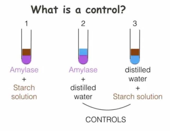
Control variables are variables whose effects are held constant (literally, ‘controlled for’) while we examine the relationship between the IV and the DV.
Sources of Spuriousness
The mere fact that two variables are empirically associated does not mean that there is necessarily any causal connection between them
Think: pollution and literacy rates, number of firefighters and amount of fire damage, migration of storks and the birth rate in Sweden…
These are all (silly!) examples of spurious relationships. In each case, the observed relationship can be explained by the fact that the variables share a common cause
A source of spuriousness variable is a variable that causes both the IV and the DV. Remove the common cause and the observed relationship between the IV and the DV will weaken or disappear. If you overlook SS, you risk research being completely wrong.
To identify a potential (SS) source of spuriousness, ask yourself (1) whether there is any variable that might be a cause of both the IV and the DV and (2) whether that variable acts directly on the DV as well as on the IV.
If the variable only acts directly on the IV, it is not a potential source of spuriousness. It is simply an antecedent. An antecedent is not a control variable.
Sources of Spuriousness II
- To identify a potential (SS) source of spuriousness, ask yourself (1) whether these is any variable that might be a cause of both the IV and the DV and (2) whether that variable acts directly on the DV as well as on the IV.
- If the variable only acts directly on the IV, it is not a potential source of spuriousness. It is simply an antecedent. An antecedent is not a control variables.
SS à IV à DV
- Examples; The higher people’s income, the great their interest in politics.
- BUT it could be spurious: education could be a source of spuriousness:
Income à Interest in Politics
Education (spuriousness)
Education à Support for Feminism
Generation (spuriousness)
- Some variables won’t have a spurious independent variable: ethnicity religion.
Intervening Variables I
Once we have eliminated potential sources of spuriousness, we must test for plausible intervening variables
Intervening variables are variables that mediate the relationship between the IV and the DV. An intervening variable provides an explanation of why the IV affects the DV
The intervening variable corresponds to the assumed causal mechanism. The DV is related to the IV because the IV affects the intervening variable and the intervening variable, in turn, affects the DV.
IV-> Intervening->DV
To identify plausible intervening variables, ask yourself why you think the IV would have a causal impact on the DV.
-can be more than one potential rationale. Intervening variable validates causal thinking.
Intervening Variables II:
- To identify plausible intervening variables, ask yourself why you thinking the IV would have a causal impact on the DV.
- Examples:
- Women are more likely than men to favour an increase in social spending.
- GENDER à RELIANCE ON THE WELFARE STATE à FAVOUR INCREASE IN SOCIAL SPENDING
- The lower people’s income the more politically alienated they will be.
- PERSONAL INCOME à PERCEPTION OF SYSTEM RESPONSIVENESS à Political ALIENATION
Conditional variables I.
-trickiest and most common. What will happen to relation btwn IV and DV?
Once we have eliminated plausible sources of spuriousness and verified the assumed causal mechanism, we need to specify the conditions under which the hypothesized relationship holds.
Ideally, we want there to be as few conditions as possible because the aim is to come up with a generalization.
Conditional variables are variables that literally condition the relationship between the IV and the DV by affecting:
(1) the strength of the relationship between the IV and the DV (i.e. how well do values of the IV predict values of the DV?) and
(2) the form of the relationship between the IV and the DV (i.e. which values of the DV tend to be associated with which values of the IV?)
-focus is always on its effect on hypothesize relation btwn IV and DV (in every category of the conditional variable. Ex) category = religion. Christian, Muslim, Atheist. Or important, not important, somewhat)
To identify plausible (CV) conditional variables, ask yourself whether there are some sorts of people who are likely to take a particular value on the DV regardless of their value on the IV.
Note: the focus is always on how the hypothesized relationship is affected by different values of the conditional variable.
There are basically three types of variables that typically condition relationships:
(1) variables that specify the relationship in terms of interest, knowledge or concern. Example (interest, knowledge or concern):
Catholics are more likely to oppose abortion than Protestants.
If CV = attends church then: religious affiliation -> support for abortion.
If CV = not attend, then religious affiliation -> does not support
(2) variables that specify the relationship in terms of place or time. (where are they from?) Example (place or time):
The higher people’s incomes, the more likely they are to participate in politics
If CV = non-rural resident, then income -> political participation
If CV = rural resident then income does not -> political participation
(3) variables that specify the relationship in terms of social background characteristics.
Examples (Social Background Characteristics):
The more religious people are, the more likely they are to oppose abortion.
If CV = male then religiosity -> views on abortion
If CV = female then religiosity does not -> abortion
Stages in Data Analysis:
Test hypothesis –> Test for Spuriousness –> If non-spurious, test for intervening variables –> test for conditional variables.

Topic 6: Research Problems and the Research Process
OVERVIEW
- What is a research problem?
- Maximizing generality
- Why is generality important?
- Overview of the research process
- Stages in data analysis
What is a research problem?
A properly formulated research problem should take the form of a question: how is concept A related to concept B?
Examples:
How is income inequality related to regime type?
How is moral traditionalism related to gender?
How is civic engagement related to social networks?
Maximizing Generality
Aim for an abstract and comprehensive formulation rather than a narrow and specific one.
Example: you want to explain support for the Parti-Québécois.
A possible formulation of the research problem:
How is concern for the future of the French language related to support for the PQ?
A better formulation of the research problem:
How is cultural insecurity related to support for nationalist movements?
Why is Generality Important?
- Goal of the empirical method is to come up with a generalization.
- Greater contribution because findings will have implications beyond the particular puzzle that motivated the research.
Access to a more diverse theoretical and empirical literature in developing a tentative answer to the research question.
The Research Process
Find a puzzle of anomally –> Formulate the research problem. How is A related to B? –> Develop hypothesis explaining how and why A and B are related –> Identify plausible sources of spuriousness, intervening variables and conditional variables. –> Choose indicators to represent the IV, DV and control variables (‘operationalization’) –> Collect and analyze the data.
Stages in Data Analysis:
Test hypothesis –> Test for Spuriousness –> If non-spurious, test for intervening variables –> test for conditional variables.

Topic 7: From concepts to indicators
Overview:
- What is ‘operationalization’?
- What are indicators?
- Converting a proposition into a testable form
- Key properties of an operational definition
An example: operationalizing ‘socio-economic status’
What is Operationalization?
Operationalization is the process of selecting observable phenomena to represent abstract concepts.
When we operationalize a concept we literally specify the operations that have to be performed in order to establish which category of the concept is present (classificatory concepts) or the extent to which the concept is present (comparative or quantitative concepts).
The end product of this process is the specification of a set of indicators.
What are indicators?
Indicators are observable properties that indicate which category of the concept is present or the extent to which the concept is present.
In order to test our theory, we examine whether our indicators are related in the way that our theory would predict.
The predicted relationship is stated in the form of a working hypothesis.
The working hypothesis is logically implied by one of the propositions that make up our theory. Because it is logically implied by the proposition, evidence about the validity of the working hypothesis can be taken as evidence about the validity of the proposition.
Converting a Proposition into a Testable Form I
Concept -> proposition -> concept
Variable -> hypothesis -> variable
Indicator -> working hypothesis -> indicator
Converting a Proposition into a Testable Form I
Just as it is possible to represent one concept by several different variables, so it is possible—and desirable—to represent one variable by several different indicators.
Concept: variable (2 or more): Indicator (2 or more each).
Key Properties of an Operational Definition
The operational definition specifies the indicators by setting out the procedures that have to be followed in order to represent the concept empirically.
A properly framed operational definition:
-adds precision to concepts
-makes propositions publicly testable
This ensures that our knowledge claims are transmissible and makes replication possible.
An Example: Operationalizing ‘Socio-Economic Status’
The first step in representing a concept empirically is to provide a nominal definition that sets out clearly and precisely what you mean by your concept:
Socio-Economic Status: ‘a person’s relative location in a hierarchy of material advantage’.
Socio economic status: 1. Income -> earnings from employment, annual household income
- wealth: value of assets, home ownership

Topic Eight: Questionnaire Design and Interviewing
Overview:
-The function of a questionnaire
-The importance of pilot work and pre-testing
-Open-ended versus close-ended questions
-Advantages and disadvantages of close-ended questions
-Advantages and disadvantages of open-ended questions
-Ordering the questions
-Common errors in question wording
-A checklist for identifying problems in the pre-test
–important to know what makes good survey research
-simply a formal way of asking people questions: attitude, beliefs, background, opinions
-follows a highly standardized structured, thought out sequence
The Function of a Questionnaire
-The function of a questionnaire is to enable us to represent our variables empirically.
-Respondents’ coded responses to our questions serve as our indicators.
-The first step in designing a questionnaire is to identify all of the variables that we want to represent (i.e. independent variables, dependent variables, control variables).
Do not pose hypothesis directly. One question cannot operationalize two variables.
-We must always keep in mind why we are asking a given question and what we propose to do with the answers.
-A question should never pose a hypothesis directly. We test our hypotheses by examining whether people’s answers to different questions go together in the way that our hypotheses predicted.
The Importance of Pilot Work
Second step: pilot work
Careful pilot work is essential in designing a good questionnaire. Background work to prepare surveys.
Pilot work can involve:
-lengthy unstructured interviews with people typical of those we want to study
-talks with key informants
-reading widely about the topic in newspapers, magazines and on-line in order to get a sense of the range of opinion.
The Importance of Pre-testing
Third step: draft a questionnaire
Fourth step: pretest questionnaire
Once a questionnaire has been drafted, it should be pre-tested using respondents who are as similar as possible to those we plan to survey
-ideally, people you test are typical of group you want to represent.
-purposif/judgmental sampling: use knowledge of population to choose subjects
-pretest very important & often humbling
Pre-testing can help with:
- identifying flawed questions
- improving question wording
- ordering questions
- determining the length of time it takes to answer the questionnaire or interview the respondents
- assessing whether responses are affected by characteristics of the interviewer
- improving the wording of the survey introduction (who am I, what I’m doing, why I’m doing it. Doesn’t say what hypotheses are.)
Open-Ended versus Close-Ended Questions
Surveys typically include a small number of open-ended questions and a larger number of close-ended questions.
In open-ended questions, only the wording of the question is fixed. The respondent is free to answer in his or her own words. The interviewer must record the answer word-for-word, w/out abbreviations.
In close-ended questions, the wording of both the question and the possible response categories is fixed. The respondent selects one answer from a list of pre-specified alternatives. (don’t read out “other”, but should be present in case they say something else)
Advantages of Close-Ended Questions
- help to ensure comparability among respondents
- ensure that responses are relevant. Allows comparison
- leave little to the discretion of the interviewer. Respondent has control over classification of their answer.
- take relatively little interviewing time: quick to ask & answer
- easy to code, process, and analyze the responses
- give respondents a useful checklist of possibilities
- help people who are not very articulate to express an opinion
Disadvantages of Close-Ended Questions
- may prompt people to answer even though they do not have an opinion (preferable not to offer “no opinion” but have it on questionnaire. Difference btwn don’t know and no answer.
- may channel people’s thinking, producing responses that do not really reflect their opinion. Bias results.
- may overlook some important possible responses
- may result in a loss of rapport with respondents: throw in open-ended to engage people
- misunderstanding (if using terms that could be difficult, provide definition for interviewers. Don’t adlib.)
The responses to close-ended questions must always be interpreted in light of the pre-set alternatives that were offered to respondents.
Advantages and Disadvantages of Open-Ended Questions
Advantages
Open-ended questions avoid the disadvantages of close-ended questions. They can also provide rich contextual material, often of an unexpected nature. (quotes can make report more interesting).
-avoid putting ideas in people’s heads
-can engage people
Disadvantages
Open-ended questions are easy to ask—but they are difficult to answer and still more difficult to analyze. Open-ended questions:
- take up more interviewing time and impose a heavier burden on the interviewer
- increase the possibility of interviewer bias if the interviewer ends up paraphrasing the responses
- require more processing
- increase the possibility of researcher bias since the responses have to be coded into categories for the purpose of analysis (must reduce to a set of numbers. Introduce risk of bias. Getting others to code for intersubjectivity is time consuming and expensive.)
- the classification of responses may misrepresent the respondent’s opinion. Respondent’s have no control over how their response is used.
- transmissibility and hence replicability may be compromised by the coding operation
- respondents may give answers that are irrelevant. Solution: use open-ended in pilot study, then create close ended with answers. Some amount of info lost, less likely to overlook important alternative.
-close-ended response categories must be mutually exclusive and cover every category.
-avoid multiple answers (which is closest, comes closest to point of view)
-can have open & close-ended versions of same question, spread out in survey. Always open first.
Ordering the Questions
Question sequence is just as important as question wording. The order in which questions are asked can affect the responses that are given:
- make sure that open-ended and close-ended versions of the same question are widely separated and that the open-ended version is asked first. (sufficiently separated)
- if two questions are asked about the same topic, make sure that the first question asked will not colour responses to the subsequent question. Change order or separate questions.
- avoid posing sensitive questions too early in the questionnaire.
- begin with non-threatening questions that engage the respondent’s interest and seem related to the stated purpose of the survey. Help create rapport.
- ensure some variety in the format of the questions in order to hold the respondent’s attention.
-when reading over questionnaire, try to think how you would react. Not intimidating. Shouldn’t seem like a test
-have you unwittingly made your own views obvious and favoured a particular position?
-worded in a friendly, conversational way. Should seem natural.
-writing questions is likened to catching a particularly elusive fish.
-making assumptions that everyone understands the question the same way. The way you intended, assuming people have necessary information. Make questions unambiguous. Problem: people will express non-attitudes.
-if problems writing questions, often b/c not completely clear on topic concept. Importance of nominal definition.
Common Errors in Question Wording
‘Do you agree or disagree with the supposition that continued constitutional uncertainty will be detrimental to the Quebec economy?’
Error #1: the question uses language that may be unfamiliar to many respondents. The wording should be geared to the expected level of sophistication of the respondents.
‘Please tell me whether you strongly agree, somewhat agree, somewhat disagree or strongly disagree with the following statements:
People like me have no say in what the government does
The government doesn’t care what people like me think’
Error #2: the wording of the statements is vague (the federal government? the provincial government? the municipal government?) Questions must always be worded as clearly as possible. (time, place, lvl of govt)
‘It doesn’t matter which party is in power, there isn’t much governments can do these days about basic problems’
Error #3: this is a double-barreled question. A respondent could agree with one part of the question and disagree with the other.
‘In federal politics, do you usually think of yourself as being on the left, on the right, or in the center?’
Error #4: this question assumes that the respondent understands the terminology of left and right.
‘Would you favor or oppose extending the North American Free Trade Agreement to include other countries?”’
Error #5: this question assumes that respondents are competent to answer. Also doesn’t say to what other countries. Solution: filter question: Do you happen to know what NAFTA is? People will want to answer even if they don’t know what it is (ex, fictitious topics). Lack of information.
‘Should welfare benefits be based on any relationship of economic dependency where people are living together, such as elderly siblings living together or a parent and adult child living together or should welfare benefits only be available to those who are single or married and/or have children under the age of 18 years?’
Error #6 this question is too wordy. In a self-administered survey, a question should contain no more than 20 words. In a face-to-face or telephone survey, it must be possible to ask the question comfortably in a single breath.
‘Do you agree that gay marriages should be legally recognized in Canada?’
Error #7: this is a leading question that encourages respondents to agree. The problem could be avoided by adding ‘or disagree. Especially important to avoid in regard to sensitive topics.
‘Canada has an obligation to see that its less fortunate citizens are given a decent standard of living’.
Error #8: this question is leading because it uses emotionally-laden language e.g. ‘less fortunate’, ‘decent’. Can also be leading by identifying with prestigious person or institution like Supreme Court, or w/someone who is disliked.
How often have you read about politics in the newspaper during the last week?
Error #9: this question is susceptible to social desirability bias because it seems to assume that the respondent has read the newspaper at least once during the previous week. People answer through filter of what makes them look good. “Have you had time to read the newspaper in the last week?”
-don’t abbreviate
-no more than 1 question per line
-open-ended must have space to write
-clear instructions
-informed consent
-privacy/confidentiality
A Checklist for Identifying Problems in the Pre-Test
- Did close-ended questions elicit a range of opinion or did most respondents choose the same response category?
- Do the responses tell you what you need to know?
- Did most respondents choose ‘agree’ (the question was too bland -> should protect nature) or did most respondents choose ‘disagree’ (the question was too strongly worded -> abortion is murder)?
- Did respondents have problems understanding a question? Were there a lot of don’t knows? (if they don’t get it, ask it again and move on)
- Did several respondents refuse to answer the same question?
- Did open-ended questions elicit too many irrelevant answers? (can you code responses)
- Did open-ended questions produce yes/no or very brief responses? Add a probe. (best probe is silence, pen poised to record)
Topic 9: Content Analysis
Overview:
What is content analysis?
What can we analyze?
What questions can we answer?
Selecting the communications
Substantive content analysis
Substantive content analysis: coding manifest content
Substantive content analysis: coding latent content
Structural content analysis
Strengths of content analysis
Weaknesses of content analysis
What is content analysis?
-involves the analysis of any form of communication
-communications form the basis for drawing inferences about causal relations
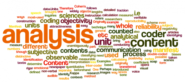
-Content analysis is ‘any technique for making inferences by systematically and objectively identifying specified characteristics of communications’. (Holsti)
-Systematically means that content is included or excluded according to consistently applied criteria.
-Objectively requires that the identification be based on explicit rules. The categories used for coding content must be defined clearly enough and precisely enough that another researcher could apply them to the same content and obtain the same results
(transmissibility+replicability=intersubjectivity).
What can we analyze?
Content analysis can be performed on virtually any form of communication (books, magazines, poems, songs, speeches, diplomatic exchanges, videos, paintings…) provided:
- there is a physical record of the communication.
- the researcher can obtain access to that record
A content analysis can focus on one or more of the following questions: ‘who says what, to whom, why, how, and with what effect?’ (Lasswell)
-who/why: inferences about sender of the communication, causes or antecedents. Why does it take the form that it does?
-with what effect: inferences about effects on person(s) who receives it
What questions can we answer?
Content analysis can be used to:
- test hypotheses about the characteristics or attributes of the communications themselves (what? how?)
- make inferences about the communicator and/or the causes or antecedents of the communication (who? why?)
- make inferences about the effect of the communication on the recipient(s) (with what effect?)
Rules of Content analysis
i.specify rules for selecting communications that will be analyzed
- specify characteristics you will analyze (what aspects of content)
iii. formulate rules for identifying characteristics when they appear
- apply the coding scheme to the selected communications
Selecting the communications
The first step is to define the universe of communications to be analyzed by defining criteria for inclusion.
Typical criteria include:
- the type of communication
- the location, frequency, minimum size or length of the communication
- the distribution of the communication
- the time period
- the parties to the communication (if communication is two-way or multi-way)
If too many communications meet the specified criteria, a sampling plan must be specified in order to make a representative selection.
-if study is comparative, must choose comparable communications. Control in content analysis is the way communications are chosen (as similar as possible except one thing).
Type of Analysis (substantive vs structural)
Substantive content analysis
-In a substantive content analysis, the focus is on the substantive content of the communication—what has been said or written.
-A substantive content analysis is essentially a coding operation.
-The researcher codes—or classifies—the content of the selected communications according to a pre-defined conceptual framework
Examples:
- coding newspapers editorials according to their ideological leaning
- coding campaign coverage according to whether it deals with matters of style or substance
Substantive Content Analysis: Coding Manifest Content
-A substantive content analysis can involve coding manifest content and/or latent content
-Coding manifest content means coding the visible surface content i.e. the objectively identifiable characteristics of the communication
-list of words/phrases that are empirical counterparts to your concept (the hard part!)
-important to relate it to some sort of base -> longer means more likely to use particular words
-Example: choosing certain words or phrases as indicators of the values of key concepts and then simply counting how often those words or phrases occur within each communication.
Advantages:
- Ease
- Replicability
- Reliability (consistency)
Intersubjectivity?
Disadvantages
- meaning depends on context
- loss of nuance and sublety of meaning
-possible that word is being used in an unexpected way (irony, sarcasm)
-validity: are we really measuring what we think we’re measuring?
Substantive Content Analysis: Coding Latent Content
Coding latent content involves coding the underlying meaning. (tone of media, etc)
Example:
- reading an entire newspaper editorial and making a judgment as to its overall ideological leaning.
reading an entire newspaper story and making a judgment as to whether the person covered is reflected in a positive, negative, or neutral light.
Advantages
(1) less loss of meaning and thus higher validity.
Disadvantages
(1) requires the researcher to make judgments and infer meaning, thus increasing risk of bias.
(2) lower reliability.-> differences in judgment
(3) lower transmissibility and hence replicability. -> cannot communicate to a reader exactly how judgement was made
-researcher is making judgments about meaning, which may be influenced by own values
Solution: take 1 hypothesis & test it different ways. More compelling, more experience w/ pros and cons of content analysis. Test hypothesis as many ways as possible.
-strive for high intercoder reliability (2 people recode independently, 90% similarity)
-use all 3 methods
Structural Content Analysis
A structural content analysis focuses on physical measurement of content.(time, space)
Examples:
- how much space does a newspaper accord a given issue (number of columns, number of paragraphs, etc.)?
- how much prominence does a newspaper accord a given issue (size of headline, placement in the newspaper, presence of a photograph, etc.)?
- how many minutes does a news broadcast give to stories about each political party?
- Column inches, seconds of airtime, order of stories, pages, paragraphs, size of headline, photograph= measures of prominence
Measurements of space and time must always be related to the total size/length of the communication
-standardize: relative to size w/same paper, not compare headline size in 2 papers
Advantages
- reliability
- replicability -easy to explain methods
Disadvantages
- loss of nuance & subtlety of meaning
-less valid: can you really represent subtle nuanced ideas by counting/measuring?
Strengths of Content Analysis
-economy
-generalizability (external validity). Representative, more confidence.
-safety: risk of missing something, time, etc not existant here. You can recode.
-ability to study historical events or political actors: asking people means you get answers they think now, not what they thought then
-ability to study inaccessibly political actors (supreme court justices)
-unobtrusive (non-reactive)
-reliability: highly reliable way of doing research, consistent results (structural, manifest)
-few ethical dilemmas. Communications already been produced, won’t harm or embarrass people.
Weaknesses of content analysis
-requires a physical record of communication
-need access to communications
-loss of meaning (low validity): are we measuring what we think we’re measuring?
-risky to infer motivations—political actors do not necessarily mean what they write or say. (Take into account purpose of communication if asking why)
-laborious and tedious
-subjective bias -> important elements of subjectivity (latent analysis: making judgements, inferences about meaning)
-> no one best way of doing content analysis. Do all 3.
Major Coding Categories
-warfare: a battle royal, political equivalent of heat seeking missiles, fighting a war on several fronts, a night of political skirmishes, took a torpedo in the boilers, master of the blindside attack
-general violence: a goold old-fashioned free-for-all, one hell of a fight, assailants in the alley
-sports and games: contestants squared off, left on the mat, knockout blow
-theatre and showbiz: a dress rehearsal, got equal billing, put their figures in the spotlight
-natural phenomena: nothing earth-shattering, an avalanche of opinion
-other
Coding Statements
-descriptive: present the who, what, where, when, without any meaningful qualification or elaboration
-analytical: draw inferences or reach conclusions (typically about the causes of the behaviour or event) based on fact not observed
-evaluative: make judgments about how well the person being reported on performed
Topic 10: Measurement
Overview:
What is measurement?
Rules and levels of measurement
Nominal-level measurement
Ordinal-level measurement
Interval-level measurement
Ratio-level measurement
What is Measurement?
-foundation of statistics
Measurement is the process of assigning numerals to observations according to rules.
These numerals are referred to as the values of the variable we are measuring (not numbers, but numberals, simply symbols or labels whereas numbers have quantitative meaning).
Measurement can be qualitative or quantitative.
If we want to measure something, we have to make up a set of rules that specify how the numerals are to be assigned to our observations.
Rules and Levels of Measurement
-The rules determine the level, or quality, of measurement achieved. <- most important part of definition.
-The level of measurement determines what kinds of statistical tests can be performed on the resulting data.
-The level of measurement that can be achieved depends on:
- the nature of the property being measured
- the choice of data collection procedures
-The general rule is to aim for the highest possible level of measurement because higher levels of measurement enable us to perform more powerful and more varied tests.
-The rules can provide a basis for classifying, ordering or quantifying our observations.
-no hierarchical order, can substitute any numeral for any other numeral. All they indicate is that the categories are different.
4 Levels: NOIR
Nominal-level measurement
Ordinal-level measurement
Interval-level measurement
Ratio-level measurement
Nominal-level measurement
-Nominal-level measurement represents the lowest level of measurement, most primitive, least information
-Nominal measurement involves classifying a variable into two or more (predefined) categories and then sorting our observations into the appropriate category.
-The numerals simply serve to label the categories. They have no quantitative meaning. Words or symbols could perform the same function. There is no hierarchy among the categories and the categories cannot be related to one another numerically. The categories are interchangeable.
-classify
-Rule: do not assign the same numeral to different categories or different numerals to the same category. The categories must be exhaustive and mutually exclusive.
Ex) sex, religion, ethnic origin, language
Ordinal-Level Measurement
-Ordinal-level measurement involves classifying a variable into a set of ordered categories and then sorting our observations into the appropriate category according to whether they have more or less of the property being measured. Allows ordering and classifying. Notion of hierarchy.
-The categories stand in a hierarchical relationship to one another and the numerals serve to indicate the order of the categories. Numerals stand for relative amount of the property.
-classify, order
-more useful, direction of relation btwn variables
-With ordinal-level measurement, we can say only that one observation has more of the property than another. We can not say how much more.
Ex) social class, strength of party loyalty, interest in politics
Interval-Level Measurement
-Interval-level measurement involves classifying a variable into a set of ordered categories that have an equal interval (fixed and known interval) between them and then sorting our observations into the appropriate category according to how much of the property they possess.
-There is a fixed and known interval (or distance) between each category and the numerals have quantitative meaning. They indicate how much of the property each observation has (actual amount).
-Classify, order, meaningful distances.
-With interval-level measurement, we can say not only that one observation has more of the property than another, we can also say how much more.
-BUT we cannot say that one observation has twice as much of the property than another observation. Zero is arbitrary.
Ex) celcius and farenheit scales of temperature
Ratio-Level Measurement (highest)
-The only difference between ratio-level measurement and interval-level measurement is the presence of a non-arbitrary zero point.
-A non-arbitrary zero point means that zero indicates the absence of the property being measured.
-Now we can say that one observation has twice as much of the property as another observation.
-Any property than can be represented by counting can be measured at the ratio-level.
-classify, order, meaningful distance, non-arbitrary zero
Ex) income, years of schooling, gross national product, number of alliances, turnout to vote
-in poli sci, few things are above the ordinal level. Stretches credulity to believe that we could come up with equal units of collectivism or alienation.
-anything that can be measured at a higher lvl can be measured at a lower lvl
-always try to achieve highest lvl of measurement. Constrained by technique used to collect data.
Topic 11: Statistics: Describing Variables
Overview:
Descriptive versus inferential statistics
Univariate, bivariate and multivariate statistics
Univariate descriptive statistics
Describing a distribution
Measuring central tendency
Measuring dispersion
Descriptive versus Inferential Statistics
Descriptive statistics are used to describe characteristics of a population or a sample.
Inferential statistics are used to generalize from a sample to the population from which the sample was drawn. They are called ‘inferential’ because they involve using a sample to make inferences about the population.
Univariate, Bivariate and Multivariate Statistics
Univariate statistics are used when we want to describe (descriptive) or make inferences about (inferential) the values of a single variable.
Bivariate statistics are used when we want to describe (descriptive) or make inferences about (inferential) the relationship between the values of two variables.
Multivariate statistics are used when we want to describe (descriptive) or make inferences about (inferential) the relationship among the values of three or more variables.
-can all be descriptive or inferential
Univariate Descriptive Statistics
Data analysis begins by describing three characteristics of each variable under study:
- the distribution : how many cases take each value?
- the central tendency: which is the most typical value? best represents a typical case
- the dispersion: how much do values vary? how spread out are cases across the possible categories? If there is much dispersion, measure of central tendency may be misleading.
-frequency value tells us how many cases take each of the possible values. Records the frequency with which each possible value occurs.
Describing a Distribution I
Knowing how the observations are distributed across the various possible values of the variable is important because many statistical procedures make assumptions about the distribution. If those assumptions are not met, the procedure is not appropriate.
A frequency distribution is simply a list of the number of observations in each category of the variable. It is called a frequency distribution because it displays the frequency with which each possible value occurs.
-frequency value tells us how many cases take each of the possible values. Records the frequency with which each possible value occurs.
Describing a distribution:
Raw frequencies (how many cases took off diff possible values)
-title informative, tell us variable for which data is being presented. Not interpret table
-source: name source
-footnote
-totals are difficult to compare, translate into %
-gives a relative idea of what to expect in the rest of the population
-gives a consistent base to make comparisons
-never report % w/out also reporting total # of cases in survey. Makes data meaningful.
– no % w/fewer than 20 cases: present raw frequency
-if data come from a sample, round off percentages to the nearest whole number, should assume that there is error.
-round up to .6-.9. round down .1-.4. with 0.5, round to nearest even number.
-99, 100, and 101% are acceptable totals. Can add note saying that numbers may not add up to 100.
-present in form of graph or chart. Contains exact same info, but easier to visualize. More interpretable, more appealing. Pie-chart, line graph.
-tricks: truncated scale to make things look better/worse. Always check the scaling.
-need to check distribution to make sure that its appropriate to use a particular statistic
Interval/ratio: not simply numerals, but numbers w/quantitative meanings. Can’t use bar or pie chart. To present distribution, must collapse lvls of variables into small groups.
-guidelines: 1. At least 6, but no more than 20 intervals. Lose to much info about distribution if too small, but more than 20 defeats the purpose of creating class intervals & data is not readily accessible.
- intervals must all have same width, encompass same # of values to be comparable (can have larger open-ended category at the end)
- don’t want them to be too wide. Want to be able to consider every case within a given interval to be similar, makes sense to treat cases within the interval as the same.
- must be exhaustive and mutually exclusive.
Describing a distribution: interval lvl data
-create a line graph.
-the only pts w. any info are the dots. Connect to remind reader that original distribution was continuous.
,relative frequencies, bar charts, pie-chart, interval level data,
Central Tendency versus Dispersion
A measure of central tendency indicates the most typical value, the one value that best represents the entire distribution
A measure of dispersion tells us just how typical that value really is by indicating the extent to which observations are concentrated in a few categories of the variable or spread out among all of the categories.
-evaluating central tendency. Important for evaluating sample size. Don’t want to only describe variables (see if covary in predicted ways)
-2 distributions could have similar central tendency, but be very different. Use more than one measure.
A measure of dispersion tells us how much the values of the variable vary. Knowing the amount of dispersion is important because:
- the appropriate sample size is highly dependent on the amount of variation in the population. The greater the variation, the larger the sample will need to be.
- we cannot measure covariation unless both variables do vary.
Measuring Central Tendency and Dispersion (Nominal-Level)
The mode is the most frequently occurring value—the category of the variable that contains the greatest number of cases. The only operation required is counting.
The proportion of cases that do not fall in the modal category tells us just how typical the modal value is. This is what Mannheim and Rich call the variation ratio.
-bimodal distribution: 2 are tied for most cases
V= f nonmodal
N
-dispersion: wht % of people were not in the modal category. The proportion who do not fall in the modal category tells us how typical the modal value is. Manheim and Rich call: variation ratio -> the lower the variation ratio, the more typical and meaningful the mode.
– in the case of bimodal or multimodal cases, select on mode arbitrarily.
Measuring Central Tendency and Dispersion (Ordinal-Level) I
Central Tendency:
-always present categories in order, natural order, should retain it
-central tendency based on order or relative position
The median is the value taken by the middle case in a distribution. It has the same number of cases above and below it. If even # of cases, take average of the two middle cases.
-cumulative frequency: eliminating raw frequency, tells # of cases that took that value or lower.
Dispersion:
The range simply indicates the highest and lowest values taken by the cases. Problem: could overstate variability. Range doesn’t tell us anything about how things are distributed btwn points.
The inter-quantile range is the range of values taken by the middle 50 percent of cases—inter-quantile because the endpoints are a quantile above and below the median value.
Measuring Central Tendency (Interval and Ratio-Level) I
The measure of central tendency for interval- and ratio-level data is the mean (or average value). Simply sum the values and divide by the number of cases:
Fall term grades: 70 75 78 82 85
GPA (or mean grade) = 78
-The mean is the preferred measure of central tendency because it takes into account the distance (or intervals) between cases. The fact that there are fixed and known intervals between values enables us to add and divide the values.
-The mean is sensitive to the presence of a small number of cases with extreme values:
When an interval-level distribution has a few cases with extreme values, the median should be used instead.
- The mean is sensitive to the presence of a small number of cases with extreme values: 26,000. 28,000. 29,000. 32,000, 34,000, 36,000: mean = 31,000 median=32,000
- Group #2 15,000. 18,000/ 19,000/ 22,000/ 23,000/ 25,000/ 95,000 mean=31,000 median 22,000
-Because the mean is subject to distortion, the mean value should always be presented along with the appropriate measure of dispersion.
-problematic when a few values are extreme cases. Mean take account of how far each case is from the others.
Measuring Dispersion (Interval- and Ratio-level) II
The standard deviation is the appropriate measure of dispersion at the interval-level because it takes account of every value and the distance between values in determining the amount of variability.
The standard deviation will be zero if—and only if—each and every case has the same value as the mean. The more cases deviate from the mean, the larger the standard deviation will be.
We cannot use the standard deviation to compare the amount of dispersion in two distributions that use different units of measurement (e.g. dollars and years) because the standard deviation will reflect both the dispersion and the units of measurement.
N= the number of cases, Xi = the value of each individual case, X= the mean see page 264.
Calculating Standardized Scores or Z-Values
-If we want to compare the relative position of two cases on the same variable or the relative values of the same case on two different variables like annual income and years of schooling, we can standardize the values by converting them into Z-scores.
The Z score allows us to compare scores that are based on very different units of measurement (for example, age measured in number of years and height measured in inches). -Z-scores tell us the exact number of standard deviation units any particular case lies above or below the mean:
Zi = (Xi – X)/S
where Xi is the value for each case, X is the mean value and S is the standard deviation.
Example: person1 has an annual income of $80,000 and person2 has an annual income of $30,000. The mean annual income in their community is $50,000 and the standard deviation is $20,000
Z1 = ($80,000 – $50,000)/$20,000 = 1.5
Z2 = ($30,000 – $50,000)/$20,000 = – 1
Topic Twelve: Statistics — Estimating Sampling Error and Sample Size
Overview:
What is sampling error?
What are probability distributions?
Interpreting normal distributions
What is a sampling distribution?
The sampling distribution of the sample means
The central limit theorem
Estimating confidence intervals around a sample mean
Estimating sample size—means
Estimating confidence intervals around a sample proportion
Estimating sample size–proportions
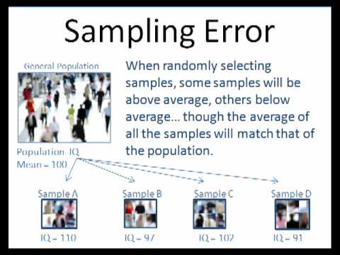
What is sampling error?
No matter how carefully a sample is selected, there is always the possibility of sampling error (i.e. some discrepancy between our sample value and the true population value).
We cannot determine the amount of sampling error directly because we typically don’t know the true population value. But we can use inferential statistics to estimate the probable sampling error associated with any sample value. Use of probability distributions.
What are probability distributions?
Estimating sampling error involves using probability distributions.
Probability distributions are theoretical distributions that indicate the likelihood, or the probability, of certain values occurring, given certain assumptions about the nature of the distribution.
By far the most important class of probability distributions take the form of a normal distribution.
The normal distribution takes the form of a symmetrical bell-shaped curve. The mean, median and mode of normally distributed data coincide with the highest point of the curve (have the same value). Can use standard deviation to interpret distribution.
Interpreting normal distributions I
The standard deviation is used to interpret data that are normally distributed.
IF data are normally distributed, 68.3% of the cases will fall within one standard deviation of the mean of the distribution, 95.5% of the cases will fall within 2 standard deviations of the mean, and 99.7% of the cases will fall within 3 standard deviations of the mean.
These proportions are equal to the proportion of the area under the curve between these values.
Interpreting normal distributions II
We can determine the proportion of cases falling within any number of standard deviations, integer or non-integer, from the mean e.g. 83.8% of cases will fall within 1.4 standard deviations of the mean
Since we use standard deviation units and not simply the original values to interpret the normal distribution, we transform the original values into standard deviation units or Z-scores.
Z= (xi – X)/s
Z-scores tell us the exact number of standard deviation units any particular case lies above or below the mean.
If our data are normally distributed, all we have to do to estimate the probability of any range of values occurring around the mean is to convert the data into Z-scores and consult the appropriate table.
What is a sampling distribution?
The sampling distribution is a theoretical probability distribution that in actual practice would never be calculated.
The sampling distribution of the sample means is the distribution that we would obtain if:
- every conceivable sample of a certain size were drawn from the same population
- the sample means were calculated for each sample and
- the sample means were arranged in a frequency distribution.
Different cases would be included in different samples so the sample means would not all be identical (e.g. some samples would contain only the very rich and some samples would contain only the desperately poor). But:
- most sample means would tend to cluster around the true population mean value and
- this clustering around the true mean value would increase if the sample size were increased
The sampling distribution of the sample means
IF the sample size is sufficiently large (at least 30 cases), the sampling distribution of the sample means will be approximately normally distributed and the mean of the sampling distribution of the sample means will coincide with the true population mean.
-can make use of the fact that it is normally distributed, and we can use that to estimate placement of the mean.
-the standard error of the mean is equal to the standard deviation of the population, divided by the square roots of the sample size
The Central Limit Theorem
The sampling distribution is a theoretical distribution–in real life, we select only one sample. But the fact that sample means will be normally distributed enables us to evaluate the probable accuracy of our particular sample mean.
Provided that our sample (1) is randomly selected (every case has a known probability of inclusion and a non-zero probability of inclusion) and (2) has at least 30 cases, the central limit theorem tells us that we can use our knowledge of the area under the curve to estimate how probable it is that the true population mean will fall within any given range of values of our sample mean.
e.g. since we know that 95.5% of sample means will lie within 2 standard deviation units of the true population mean, we can be 95.5% confident that our sample mean will also lie within 2 standard deviations of the true population mean.
Estimating confidence Intervals around a Sample Mean I
Conventionally, we want to be 90% confident, 95% confident or 99% confident. The corresponding Z-values are 1.64, 1.96 and 2.57
i.e. we can be 90% confident that our sample mean will lie within 1.64 standard deviations of the population mean, 95% confident that it will lie within 1.96 standard deviations, and 99% confident that it will lie within 2.57 standard deviations. These ranges of values are called confidence intervals.
A confidence interval is a range of values, estimated on the basis of sample data, within which we can say, with a pre-specified degree of confidence that the true population value will lie.
-the higher the confidence lvl, the wider the confidence interval must become.
Confidence level: the likelihood that our sample is in fact representative of the larger population within the degree of accuracy we have specified.
The lower the percentage of sampling error and the greater the level of confidence, the better a piece of research will be.
The size of the confidence interval will depend on how confident we want to be that the interval does contain the true unknown population mean. The more confident we want to be, the wider the confidence interval will have to be.
Estimating confidence intervals around a sample mean II
In order to determine what 1.96 standard deviations actually means in terms of our original measurement scale (e.g. dollars, years), we need to estimate the value of the standard deviation of the sampling distribution of the sample means.
The standard error of the mean is equal to the standard deviation of the population, divided by the square root of the sample size.
This makes sense intuitively:
- the more variability there is in the population, the more variability there will be in the sample estimates.
- as the sample size increases, the variability in the sample estimates should decrease because extreme values will have less of a distorting effect on the calculation of the sample mean.
Since we typically do not know the true population standard deviation, we use our best estimate i.e. the standard deviation from our particular sample.
Estimating confidence intervals around a sample mean III
We then simply multiply our estimate of the sampling error of the mean by the Z-value associated with our chosen confidence level (1.64, 1.96 or 2.57) and we have the familiar plus or minus term:
Confidence lvl: X +- Zc.l. SX
-can be confident that something lies btwn 2 levels.
Estimating sample size I
Exactly the same concepts are used to help determine sample size. The formula for calculating the sample size simply involves rearranging the terms:
where:
E = ( Zc.l. S)/square root N
- ZL. is the Z-value associated with the desired confidence level
- S is the estimate of the population standard deviation
- E is the amount of error we are willing to tolerate (i.e. the plus or minus term)
-variability, how accurate you want to be, how confident you want to be that you are that accurate.
-what is not a factor in this calculation? Population size. What matters is how much variation there is.
-calculation of sample size: constrained by resources, by variability w/in population
Estimating sample size II
In other words, we need 3 pieces of information in order to calculate sample size:
- the amount of variability or heterogeneity in the population on the characteristic that we want to estimate. We typically do not know this, so we have to use our best estimate based on e.g. prior studies or a pilot study
- the amount of error we are willing to tolerate i.e. how wide do we want our confidence interval to be?
- the confidence level–how confident do we want to be that our sample estimate is that accurate?
The population size does not affect the sample size unless the sample is going to constitute 5 percent or more of the population
Example: to estimate mean GPA within + 2 points with a 95% level of confidence and an estimated population standard deviation of 12 points:
Estimating confidence intervals around a sample proportion
The logic is exactly the same when we want to estimate a population proportion on the basis of a sample proportion.
This time we draw on our knowledge of the fact that the sampling distribution of the sample proportions will be normally distributed and we have to calculate the standard error of the proportion.
(see 12.15)
If we have no basis for estimating the sample proportion, we should use the value that assumes the maximum amount of variability.
The maximum possible value for the standard error of the sample proportion occurs when we assume a population proportion of .5

TOPIC 13: Causal Thinking and Research Design
Overview:
Why is research design so important?
The nature of causal inferences
The classic experimental design
Internal validity
Extrinsic threats to internal validity
Intrinsic threat to internal validity
Threats to external validity
Variations on the classic experimental design
Quasi-experimental designs
-generalize causal inferences
-determine causal connection
-> our ability to do this hinges on how we design our research. Don’t rule our plausible causal interpretations.
Why is research design so important?
Purpose: to impose controlled restrictions on our observations of the empirical world.
A good research design:
- allows the researcher to draw causal inferences with confidence
- defines the domain of generalizability of those inferences
The way we structure our data-gathering strongly affects the nature of the causal interpretations we can place on the results.
The research must be designed so that we can rule out plausible alternative interpretations of the observed relationships.
The nature of causal inferences
We can never be certain that one variable ‘causes’ another–but we can increase confidence in our causal inferences if we are able to:
-demonstrate co-variation
-eliminate sources of spuriousness
-establish time order
Covariation—show that the IV and DV vary together in a patterned, consistent way (if A, then B)
NonSpuriousness — rule out the possibility that the IV and DV only co-vary because they share a common cause
Time order — show that a change in the IV preceded a change in the DV
How can we get more confident?
-don’t say what causes what. Assume there is some sort of causal influence involved
-change in value of 1 variable enhanced another’s change in value
-fundamental problem of causal inference: always has one causal influence. Demonstrate covariation, demonstrate non-spuriousness, time order.
-demonstrating covariation at the heart of hypothesis testing. Time order: demonstrate that IV occured before DV. Cause b4 effect.
-causal interpretation cannot come from data itself. However, can design research so that some outcomes are impossible and/or use statistical methods to analyze data & rule out possibilities ex-post facto. Can only do this if thought of it at research design stage.
The classic experimental design I
The classic experimental design consists of two groups: an experimental group and a control group.
These two groups are equivalent in every respect, except that the experimental group is exposed to the IV and the control group is not.
To assess the effect of differential exposure to the IV, the researcher measures the values of the DV in both groups, before and after the experimental group is exposed to the IV.
The first set of measurements is called the pre-test and the second set of measurements is called the post-test.
If the difference between the pre-test and post-test is larger in the experimental group, this is inferred to be the result of exposure to the IV.
Group
Experimental
Control
Time 1
Pretest
Pretest
Time 2
Exposure to IV
Time 3
Post-test
Post-test
Why is the classic experimental design so powerful?
The classic experimental design has 3 essential components that enable us to meet the 3 requirements for demonstrating causality:
Comparison -> covariation
Manipulation -> time order
Control -> non-spuriousness
-able to study impact of IV free of all other conflicting inferences
-unfortunately, much of what we study is not amenable to this design
-even in non-experimental research, we try to mimic this design.
Internal Validity
-absolute basic requirement of a research design
A research design has internal validity when it enables us to infer with reasonable confidence that the IV does indeed have a causal influence on the DV. Must enable to us to rule out plausible alternative causal relations.
To demonstrate internal validity, our research design must enable us to rule out other plausible causal interpretations of the observed co-variation between the IV and DV.
The factors that threaten internal validity can be classified into those that are extrinsic to the actual research and those that are intrinsic.
Extrinsic threats to internal validity
Extrinsic threats to internal validity typically arise from the way we select our cases.
They refer to selection biases that cause the experimental group and the control group to differ even before the experimental group is exposed to the IV.
If the two groups are not equivalent, then a possible explanation for any difference in the post-test results is that the two groups differed to begin with.
Intrinsic threat to internal validity I
Intrinsic threats to internal validity arise once study is under way from:
-changes in the cases being studied during the study period (history)
-flaws in the measurement procedure
-the reactive effects of being observed
There are six major intrinsic threats:
History—events may occur while the study is under way which affect values on the DV quite independently of exposure to the IV. The longer the study, the greater this threat.
Maturation—physiological and /or psychological processes may affect values on the DV quite independent of exposure to the IV
Mortality—selective dropping out from the study may cause the experimental group and the control group to differ on the post-test, quite independent of exposure to the IV.
Instrumentation—if our measuring instruments do not perform consistently, this unreliability may explain why cases differ before and after exposure to the IV.
The regression effect—if cases score atypically high or atypically low when they are pre-tested, it is likely that their scores will appear more typical when they are post-tested, quite apart from exposure to the IV.
Reactivity (‘test effect’)—the very fact of being pre-tested may cause people’s values to change, quite apart from exposure to the IV.
Countering extrinsic threats to internal validity I
Extrinsic threats are countered by ensuring that the experimental group and the control group are equivalent. (selection bias might cause groups to differ before exposure) There are 3 ways of ensuring equivalence:
Precision matching (also known as ‘pairwise matching’)—each case in the experimental group is literally matched with another case in the control group which has an identical combination of characteristics.
This method can be impractical because of the difficulty of finding matched pairs of cases.
Countering extrinsic threats to internal validity II
Frequency distribution matching—instead of matching cases on combinations of characteristics, the distribution of characteristics within each group is matched (i.e. the two groups should have the same proportion of men and women, the same average income level, the same ethno-linguistic composition, etc.)
This method is easier to achieve, don’t have to reject a lot of potential cases, but:
- the effects of any one characteristic may be conditioned by the presence of other characteristics e.g. the effects of age may differ for men and women.
- we can only match social background characteristics, but people who share the same social characteristic may differ in other ways.
- we can never be confident that we have matched on all relevant characteristics.
Countering extrinsic threats to internal validity III
Randomization—cases are assigned to the experimental group and the control group in such a way that each case has an equal probability of being assigned to either group i.e. selection is left entirely to chance. (table of random, numbers, flip a coin)
If the randomization is done properly, the two groups should be equivalent.
This method controls for numerous factors simultaneously without the researcher having to make decisions about which factors might have a confounding effect.
BUT randomization requires a large number of cases in order to work effectively.
Countering intrinsic threats to internal validity
The presence of a control group that is equivalent in every respect to the experimental group except that is not exposed to the IV counters the intrinsic threats to internal validity:
History–both groups are exposed to the same events—so any difference in their post-test values must reflect differential exposure to the IV.
Maturation–both groups undergo the same maturational processes
Mortality–selective dropping out will affect both groups equally.
Instrumentation—both groups will be equally affected by random errors in measurement.
Regression effect—both groups will be equally susceptible.
Reactivity—if the pre-test does affect values on the post-test, this will be true of both groups.
-any difference must be because of the IV because everything else has been controlled for
-unambiguous basis for knowing that change in the IV occurred before change in the DV in time
-very strong internal validity, strong basis for inferring causal relations
problem: causal relations may only apply to case that you studied -> weak external validity = weak basis for generalizing
Threats to external validity
External validity concerns the extent to which the research findings can be generalized beyond the particular cases that were studied.
There are 3 threats to external validity:
-unrepresentative cases (people who volunteer are not representative)
-the artificiality of the research setting (people do not react the same way in the real world)
-reactivity—the pre-test may sensitize participants to respond atypically to the IV
The classic design is strong on internal validity and weak on external validity.
The Solomon 3-control group design
(also known as the Solomon 4-group design)
-This design has stronger external validity because it enables the researcher to assess the reactive effects of the pre-test experience.
-enhance external validity, helps assess reactive effect of the pretest
-This design is similar to the classic experimental design but it adds two more control groups. One group is exposed to the IV, but the other group is not. Neither group is pre-tested, but both groups are post-tested.
The post-test only control group design
The Solomon 3-control group design is stronger on external validity but:
- often impractical
- too costly
Another solution is to omit the pre-test altogether. This is only possible if we are very confident that the experimental group and the control group are really equivalent.
-avoid problem of testing, but still problem w/unrepresentativeness & artificiality.
-in practice cannot maximize internal & external validity. The more generalizability, the less internal validity.
-which matters most? Internal validity. Unequivocal basis for making causal inferences. However, typically study things as they are already, can’t manipulate countries/education, etc in experiments. Studying people already exposed to IV, so must use designs that are weaker in internal validity.
Quasi-experimental designs I
Experimental designs provide the most unequivocal basis for inferring causal relationships—but political phenomena are typically not amenable to experimental manipulation.
Quasi-experimental designs attempt to use the logic of the experimental design in situations where the researcher cannot randomly assign observations to experimental and control groups or control exposure to the IV.
In this design, comparison and control are achieved statistically. Multivariate statistical analysis is the most common alternative to experimental methods of control.
Quasi-experimental designs II
-The ex post facto experiment is most common type of quasi-experimental design. It attempts to approximate the post-test only control group design by using multivariate statistical methods. Try to apply logic of experimental design after having collected data. Cross-tabulations. Compare in order to demonstrate covariation.
-The researcher collects data on the IV, the DV and any other variables that might plausibly alter or even eliminate any observed covariation between the IV and the DV.
-At the analysis stage, cases are assigned to groups depending on their values on the IV. Then the researcher compares each group’s values on the DV. Any difference is inferred to be the result of the fact that the groups differ on the IV.
-To demonstrate non-spuriousness, the cases are divided into groups based on their values on the plausible source of spuriousness variable and the researcher compares values on the IV and the DV (as above) within each group. If the IV and DV continue to covary within each group, the relationship is not spurious.
-when we examine categories, we are matching: same drawback. Researchers must decide what are relevant variables and possible SS>
-taking liberties w/notion of control, try to mimic logic of the control group
-demonstrate non-spuriousness, correlation, but can’t demonstrate time-order.
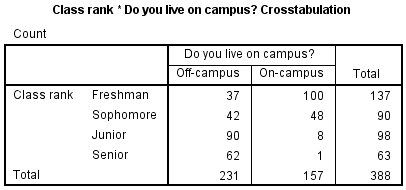
Topic Fourteen: Statistics — Cross-Tabulations and Statistical Significance
Overview
Demonstrating covariation
Creating a cross-tabulation (nominal-level relationship)
Interpreting a cross-tabulation
Statistical significance
Type I versus Type II error
Estimating the probability of Type I error
The Logic of the Chi Square Test
Calculating Chi Square
Using and Abusing the Chi Square Test
Demonstrating Covariation
Demonstrating covariation involves answering 3 questions:
ü Degree–how strong is the relationship between the IV and the DV? Strength of association. Descriptive statistics.
ü Form–which values of the DV are associated with which values of the IV? Descriptive statistics. Positive or negative relationship.
ü Statistical significance—if the data are taken from a sample, can the relationship be generalized to the population from which the sample was drawn? Could we have obtained this relationship if there wasn’t one in the population? Inferential statistics
The tests that are used to answer these questions will depend on the level of measurement of the IV and the DV. The higher the level of measurement, the more varied and the more powerful the tests that can be used.
-cases can be affected by frequency distribution.
Creating a Cross-Tabulation (nominal-level relationship) I
The first step in describing the relationship between two variables is to arrange the data so that we can get an initial visual impression of the relationship.
If both variables are measured at the nominal level, this involves arranging the data in the form of a contingency table or cross-tabulation.
-A cross-tabulation involves classifying cases according to their values on the IV and then cross-classifying them according to their values on the DV. The cells of the table display the number of cases having each possible combination of values on the IV and the DV.
-eliminate irrelevant categories (missing data). Eliminate Categories that are useless for meaningful analysis (numbers too small). Can only do this in nominal level.
-The single most common error in constructing a cross-tabulation is to percentage the wrong way.
-The cell percentages must be calculated in terms of the total number of cases in each category of the independent variable. If we are testing the hypothesis that women are less likely to vote for new right parties than men, we have to compare the % of women who voted Alliance with the % of men who voted Alliance.
-A cross-tabulation is interpreted by comparing categories of the independent variable in terms of the percentage distribution of the dependent variable i.e. we compare the % of women who voted Alliance with the % of men who voted Alliance.
-If the independent variable forms the columns of the table, the percentages are calculated by column and then the columns are compared i.e. percentage down and compare across columns.
-total in each column/row are marginal frequencies. Literally, on margin of table.
-reasons to % table: 1. If don’t have equal cases in diff IV categories, difficult to compare cell frequencies 2. Even if equal, easier to read out of 100 than other things.
-don’t use decimal to avoid a false sense of precision in %
Interpreting a Cross-Tabulation (nominal-level relationship) II
- check whether there are differences in the distribution of the DV for the different categories of the IV.
- if there are differences, check whether they are consistent with the hypothesis.
- if the percentage differences are consistent with the hypothesis, see how big they are. The larger the differences, the stronger the relationship.
- if the data come from a sample, check how likely it is that differences this large could have occurred by chance (as a result of sampling error) i.e. how confident can we be that the relationship observed in the sample exists in the population at large?
Tests:
- inter-ocular strike test: no substitute for eyeballing the table. If no difference, then there is no relation.
- Are differences continuous w/hypothesis? Is the gap the one predicted? (form)
- If % are in hypothesized direction, how big are the differences? Bigger the difference, the more impact IV is having. But % don’t have to be drastic to be meaningful.
- Statistical significance
Statistical Significance
Statistical significance indicates how likely (or probable) it is that the relationship between two variables observed in a sample might have occurred by chance and might not exist in the population from which the sample was drawn.
This probability is termed the level of statistical significance. The lower the probability, the higher the level of statistical significance. Want a low probability (.05 or less is conventional. 5% chance they don’t generalize)
A test of statistical significance is an inferential statistic. Purpose to estimate how likely it is that results occurred by chance & is not representative of population.
Type I versus Type II Error
In making inference about the whole population based on the results of a sample, we risk making one of two types of error:
- inferring that there is a relationship when none actually exists.
- inferring that there is no relationship when there really is a relationship.
The risk of Type I error is always viewed as much more serious than Type II error:
- the analogy of a court of law—just as we’d rather risk letting a guilty person go free than convicting an innocent one, so we’d rather risk missing a relationship than inferring one where none exists.
- If our sample indicates that there is no relationship, we are usually ready to accept this verdict without worrying how confident we should be.
-much harder to calculate type II error
How to calculate type I error
-rely on theoretical frequency distribution, which provides us with criteria for assessing risk of error
-theoretical now gives likelihood of each possible degree of association in a sample if there was no relation w/in population.
-chisq distribution. Chisq= appropriate w/nominal level relations, also ordinal lvl
-cross tab is interpreted by comparing categories of the IV in terms of the % distribution of the DV. (% women alliance voters with % men alliance voters)
-if the IV forms the columns, the % are calculated by column and then the columns are compared (percentage down, compare across)
-use knowledge of theoretical distribution to judge how confident we can be that results will hold in population
Estimating the Probability of Making a Type I Error
Estimating the probability of making a Type I error (i.e. determining the level of statistical significance) involves the use of a theoretical sampling distribution.
For nominal-level relationships, the appropriate sampling distribution is the Chi-square distribution. This distribution gives the likelihood of each possible degree of relationship occurring in a sample if there were no relationship in the population from which the sample was drawn.
We use this theoretical distribution to determine how likely it is that we would have found a relationship as strong as the one observed in our sample if there were really no relationship in the population.
The Logic of the Chi Square Test
- set up a null hypothesis i.e. assume that there is no relationship in the population.
- calculate the cell frequencies you would expect to observe if the null hypothesis were true.
- compare the expected cell frequencies with the observed cell frequencies — the greater the differences, the less risk of Type I error, and the bigger chisq, the more confident we can be that there is a relationship in population.
- make a partial adjustment for sample size since the absolute amount of difference between the expected and observed cell frequencies is also a function of sample size.
- calculate the degrees of freedom—the more cell there are in a table, the greater the opportunity for the observed distribution to depart from the expected distribution.
- consult the theoretical Chi Square distribution to determine the significance level (SPSS automatically does this for you).
Calculating Expected Frequencies
-To obtain the expected cell frequency for a given cell, multiply the column marginal by the row marginal and divide by the total number of cases e.g.:
-The expected cell frequency tells us how many women we would expect to vote Alliance if the vote distribution for women matched the vote distribution for the sample as a whole. (461/1357) x 100 = 34% of the sample voted Alliance—so we would expect 34% of women to vote Alliance.
Calculating Chi Square
Xsquared = (fo – fe)squared/fe
Where: fo = the frequency observed in each cell.
fe = the frequency expected in each cell
Degrees of freedom (# of columns minus one)(# of rows minus one) = 1 x 3 = 3
Chi Square = 29.2 significance level = .001
i.e. there is less than one chance in a 1,000 that we would have obtained a relationship like the one observed in our sample if there were really no relationship in the population.
-square to get rid of negative signs so that #’s don’t cancel out
-(fo-fe)squared/fe: other things being equal, the larger size, the larger the discrepancy. Therefore want to compensate for that by making a partial adjustment. Divide by expected frequency for each cell.
-only partial adjustment b/c larger samples are more reliable.
-distributional freedom: adjust for differences in the size of the table (differences btwn tables in the # of cells that they have). the more cells in a table, the more chances there are to deviate from the random model & want to adjust for this)
Chi square:
-significant at the .001 lvl (1/1000 chance)
-if relation is .006 can talk about it being borderline, approaching statistical significance
FOR EXAM: define statistical significance, name a nominal level test, describe the logic
Using and Abusing the Chi Square Test
- Chi Square assumes that the researcher has hypothesized a relationship in advance.
- Chi Square assumes that the sample was selected randomly. (non-zero chance of inclusion)
- Chi Square assumes that no more than 25 percent of the cells have an expected frequency of less than five. More of an issue if it appears to be significant, must alert reader of the problem.
- the larger the number of cases, the larger Chi Square will be since the adjustment for sample size is only partial. This is as it should be since a larger sample reduces the risk of Type I error. BUT this means that Chi Square should NEVER be used to draw conclusions about the strength of the relationship between IV and DV (since trivial relationships will attain statistical significance if the sample is large enough). Cannot compare size of chi square from one table to another
- a non-significant Chi Square does NOT mean that our sample is unrepresentative. What it usually means is that the relationship we have observed is so weak that it could easily have occurred by chance.
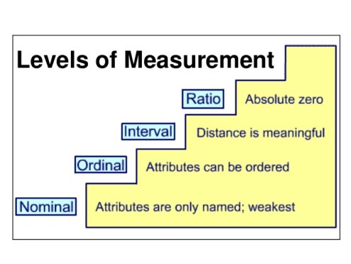
Topic Fifteen: Statistics — Nominal-Level Measures of Association
Overview
What is a Measure of Association?
What are PRE-Based Measures of Assssociation?
Calculating Lambdaa
Interpreting Lambdaa
Why Lambdaa can be misleading
What is a Measure of Asssociation?
A measure of association (or correlation coefficient) is a single number that summarizes the degree of association between two variables.
There is a wide range of measures available for describing how strongly two variables are related. Some differ in their basic approach, but even when the basic approach is similar, measures may differ with respect to:
- the type of data for which they are appropriate
- their computational details
This means that different measures of association are not directly comparable. Never compare how strong different relationships are unless the same measure of association has been used.
What are PRE-Based Measures of Association?
The logic of proportional reduction in error (PRE) provides an intuitive approach to measuring association. It involves asking: how much does knowing the values of cases on the independent variable help us improve our ability to predict their values on the dependent variable?
If two variables are perfectly related, knowing a case’s value on the IV will enable us to predict its value on the DV with complete accuracy. Conversely, if two variables are completely unrelated, knowing the value of a case on the IV will be no help at all in predicting its value on the DV.
If two variables are partially related, knowing the value of a case on the IV will be some help in predicting its value on the DV. PRE-based measures enable us to summarize that improvement in predictive ability.
Calculating Lambdaa I
Lambdaa is a PRE-based measure of association that is appropriate when one or both variables are measured at the nominal level.
Lambdaa measures how much our predictive ability is improved by knowing the values of cases on the IV. It ranges in value from .00 (no improvement) to 1.00 (perfect predictability).
If you had to guess how any one person voted, your best guess would be the modal category (Liberal).
And if you had to make the same guess for every person, you would make the fewest errors if you always guessed the modal category.
-single # that summarizes degrees of correlation btwn 2 variables
-many diff variables of association: conceptualize in different ways. Cannot compare different measures of association.
-widely used. Employ logic that is very direct literal interpretation
-lamda a = asymetrical lamda
-lamda is attractive measure of association b/c it is easily readable. Don’t want to take it that literally, not strong relationship til .50
Lamda = fi-fd/n-fd
Where fi = maximum frequency w/in each subclass or category of the IV
Fd= maximum frequency in the totals of the DV
N = number of cases
Interpreting Lambdaa
The value of Lambdaa depends on which variable is used as the predictor variable—the column variable or the row variable.
Lambdaa is asymmetric Lambda (hence the subscript), meaning that it is used when we want to predict the values of one variable based on the values of a second variable. There is also symmetric Lambda which is used when we want to summarize the degree of mutual predictability between two variables (how much does our predictive ability improve if we use each variable to predict the other?)
SPSS provides all three Lambdas—so be sure to choose the asymmetric Lambda that corresponds to your DV.
Why Lambdaa can be misleading
Lambdaa will always be zero if the modal value is the same for all categories of the IV.
-be skeptical if get .00. If modal category is the same for categories of the DV, lamda will be .00. statistic no longer giving appropriate distribution of variables.
If the modal value is the same for all categories of the IV, then Cramer’s V will be an appropriate measure to use for nominal-level relationships. Cramer’s V is based on the logic of Chi Square (i.e. it is not a PRE-based measure). It adjusts Chi Square to minimize the effects of sample size and distributional freedom(the more cells in a table, the more opportunities there are to differ from population) and to constrain the coefficient to range between .00 and 1.00.
-cannot give literal interpretation of cramer’s v. only gains meaning when comapred to diff tables & strength of association
-cannot compare cramer’s v and lamda
-not a PRE based measure.
-arrange data to get initial visual impression. Can create rank-ordering (used w/ordinal variable w/ large # of possible values. Very few cases w/ same values) or cross tabulation/contingency table. Btwn 3 & 7 values.
Topic Sixteen: Statistics — Ordinal-Level Measures of Association
Overview
Creating a cross-tabulation
Measuring association at the ordinal level
The logic of PRE at the ordinal level
Calculating Gamma
Why Gamma can be misleading
Ordinal measures of association: Tau
Choosing a measure of association
Creating a Cross-Tabulation I
The first step in describing a relationship between two variables is to arrange the data so that you can get an initial visual impression of whether there is a relationship or not. With ordinal-level data, there are two methods for doing this:
- rank orders are used when there are few cases having the same value (i.e. when there are few “ties”).
- cross-tabulations are used when there are many ties and/or when both variables have only a small number of possible values.
When cross-tabulating ordinal variables, it is important that the values of both variables be listed in the same order (e.g. from low to high, from weak to strong, etc.).
The best general indication of a relationship in a cross-tabulation between two ordinal variables is a consistent increase in the %s in one direction across the top row and in the opposite direction across the bottom row. Pattern where % increase in the top & bottom row. Do they increase in opposite directions? If so, relationship.
-always compare across rows
-focus on the gap, but not to the exclusion of what happens btwn the endpoints. Have to see a steady pattern on incrase.
Measuring Association at the Ordinal Level
Having checked that Chi Square is statistically significant (i.e. the significance level is .05 or less), the next step is to calculate a measure of association.
Measures of association at the ordinal level differ from measures of association at the nominal level in ranging from –1.00 to +1.00 (instead of .00 to 1.00).
A negative coefficient indicates that cases with high values on the IV tend to have low values on the DV (and vice versa). This indicates that there is a negative relationship between the IV and the DV.
A positive coefficient indicates that cases with high values on the IV also tend to have high values on the DV (and vice versa). This indicates that there is a positive relationship between the IV and the DV.
The Logic of PRE at the Ordinal Level I
-Gamma is an ordinal measure of association that uses the logic of proportional reduction in error.
-Association is still treated as a matter of predictability, but the nature of the predictions changes because we have ordered categories.
-With ordinal data, we are interested in measuring how much knowing the relative position (or ranking) of a pair of cases on the IV will help us to improve our ability to predict their relative position (or ranking) on the DV.
The Logic of PRE at the Ordinal Level II
There are 2 conditions under which the ranking of a pair of cases will be perfectly predictable:
- if all the cases are ranked in exactly the same order on both variables (perfect agreement) i.e. cases that have low values on the IV all have low values on the DV, etc.
- if all the cases are ranked in exactly the opposite order on both variables (perfect inversion) i.e. cases that have low values on the IV all have high values on the DV, etc.
In either case, we can predict the relative position of a pair of cases on the DV from their relative position on the IV with perfect accuracy.
The degree of predictability (or association) is a function of how close the rankings on the two variables are to either perfect agreement or perfect inversion. Both situations represent perfect association—the only difference lies in the direction of the association.
Calculating Gamma I
We use probabilistic logic to calculate and interpret Gamma.
-If two variables are in perfect agreement, the probability of drawing a positive pair (a pair of cases ranked in the same order on both variables) will be 100%:
-If two variables are in perfect inversion, the probability of drawing a negative pair (a pair of cases ranked in the opposite order on both variables) will be 100%:
-If two variables are totally unrelated, the probability of drawing a positive pair will equal the probability of drawing a negative pair.
In order to calculate the chance of drawing positive and negative pairs, we have to count the total number of positive and negative pairs.
To compute the number of positive pairs, begin with the cell in the upper leftmost corner and multiply it by the sum of the frequencies in all the cells below and to the right. Cells below will have higher values on the DV and cells to the right will have higher values on the IV. Repeat for every cell that has cells below and to the right:
To compute the number of negative pairs, begin with the cell in the upper rightmost corner and multiply it by the sum of the frequencies in all the cells below and to the left. Cells below will have higher values on the DV and cells to the left will have lower values on the IV. Repeat for every cell that has cells below and to the right:
Interpreting Gamma
If positive pairs predominate, Gamma will be positive. If negative pairs predominate, Gamma will be negative.
Gamma is literally interpreted as indicating the probability of correctly predicting the order of a pair of cases on the DV once we know their order on the IV, ignoring ties. Still using the logic of guessing.
The size of the coefficient indicates the strength of the relationship, while the sign (positive or negative) indicates the direction of the relationship. Strength of association. Clsoer to 1 = stronger.
Why Gamma can be misleading
In calculating Gamma, we ignore cases that have the same value on one or both variables (‘ties’). Cases that have the same value on one variable, but a different value on the other variable violate the notion of association. Ignoring these cases causes Gamma to overstate the degree of association.
Ordinal Measures of Association: Tau
Because Gamma can be inflated, it is preferable to use Tau. Tau does take into account cases that are tied on one variable, but not on the other (cases that are tied on both variables are consistent with the notion of association).
Like Gamma, Tau ranges in value from –1.00 to +1.00
Taub is used when both variables have the same number of values (i.e. the table is symmetrical, with an equal number of columns and rows).
Tauc is used when one variable has more values than the other variable (i.e. the table is asymmetrical, with an unequal number of columns and rows).
[There is also a Taua but this is not used with cross-tabulations since it assumes that there are no ties.]
-only use if both measures are ordinal (exception: dichotomous variables can be treated as ordinal, evne interval)
Left-right self-placement x support for free enterprise:
Gamma = .37 Taub = .23
Choosing a Measure of Association I
Gamma and Tau should only be used when both variables are measured at the ordinal level unless one or both variables is a dichotomy.
A dichotomous variable has only 2 categories (e.g. sex). As such, it satisfies the requirements for both interval-level (there is only one interval which, by definition, is equal to its self) and ordinal-level (the ordering is arbitrary but neither ordering violates the mathematical requirements) measurement
IV DV Measure of Association
nominal nominal Lambda or Cramer’s V
nominal dichotomy
nominal ordinal
dichotomy nominal
ordinal nominal
ordinal ordinal Gamma or Tau
dichotomy ordinal
ordinal dichotomy
dichotomy dichotomy
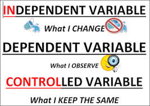
Topic Seventeen: Statistics — Examining the Effects of Control Variables
Overview
How are controls introduced?
Interpreting control variables
Sources of Spuriousness
Intervening variables
Conditional variables
Replicated relationships
How are controls introduced?
It is never enough to demonstrate covariation. We must always go on to examine the effect of other variables (‘control variables’) that might plausibly alter or even eliminate the observed covariation.
In order to determine whether some third variable affects the observed relationship between the IV and DV, we must be able to hold the effects of that variable constant and then re-examine the relationship between the IV and the DV. Note: the focus is always on what happens to the IV – DV relationship.
With nominal variables or with ordinal variables that have only a small number of possible values, we use a physical control i.e. we divide our cases into groups based on their values on the control variable and then re-examine the original relationship separately for each of these groups, using a series of cross-tabulations.
Interpreting control variables
When you do this, one of three things can happen to the original relationship:
- it can stay more or less the same in every category of the control variable (replicated relationship).
- it can weaken or disappear in every category of the control variable (spuriousness OR intervening variable). Gap smaller, measure of association smaller, no sig chisq
- it can weaken in some categories and strengthen in others or even assume different forms in different categories of the control variable (conditional variable).
Note: there is no statistical technique for distinguishing between an intervening variable and a source of spuriousness. You have to decide on substantive grounds which interpretation makes the most sense. Usually, this is decided on the basis of time order. Draw chart.
-data analysis is not just a mechanical process -> process of imparting meaning to data by interpreting them.
Source of Spuriousness I
-The first priority must be to test for spuriousness i.e. we must ask whether there is some common factor that could cause both the IV and the DV.
-If the relationship between the IV and the DV is spurious, the relationship will weaken or disappear when we control for the source of spuriousness variable (remove the common cause and the observed covariation will weaken or disappear).
-If your relationship turns out to be spurious, you should make the source of spuriousness variable your new independent variable and then test the relationship between this variable and your dependent variable. You will then test for the effects of two plausible control variables.
If the original relationship weakens in every category of the control variable, but there is still some relationship in every category (i.e. the significance level is .05 or less and the measure of association is close to .20), you have a partial source of spuriousness. In this case, you do not need to change your hypothesis because there is still some covariation even controlling for the common cause.
If there is more than one plausible source of spuriousness, you must test for these additional possibilities.
Intervening Variable I
If your relationship is not spurious (or is only partially spurious), the next priority is to test for a plausible intervening variable.
Intervening variables are variables that mediate the relationship between the IV and the DV. An intervening variable provides an explanation of why the IV affects the DV.
The intervening variable corresponds to the assumed causal mechanism. The DV is related to the IV because the IV affects the intervening variable and the intervening variable, in turn, affects the DV.
To identify plausible intervening variables, ask yourself why you think the IV would have a causal impact on the DV.
Ex) The relationship has weakened in both categories of the control variable, but it has not disappeared. This indicates that ideology is a partial intervening variable (it only explains some of the observed relationship between religious affiliation and vote choice).
Conditional variables I
Once we have eliminated plausible sources of spuriousness and verified the assumed causal mechanism, we need to specify the conditions under which the hypothesized relationship holds.
Ideally, we want there to be as few conditions as possible because the aim is to come up with a generalization.
Conditional variables are variables that literally condition the relationship between the IV and the DV by affecting:
(1) the strength of the relationship between the IV and the DV (i.e. how well do values of the IV predict values of the DV?) and
(2) the form of the relationship between the IV and the DV (i.e. which values of the DV tend to be associated with which values of the IV?)
Conditional variables II
To identify plausible conditional variables, ask yourself whether there are some sorts of people who are likely to take a particular value on the DV regardless of their value on the IV.
Note: the focus is always on how the hypothesized relationship is affected by different values of the conditional variable
There are basically three types of variables that typically condition relationships:
(1) variables that specify the relationship in terms of interest, knowledge or concern.
(2) variables that specify the relationship in terms of place or time.
(3) variables that specify the relationship in terms of social background characteristics.
Replicated relationship II
What matters is what happens to the differences across the columns. Even though the cell percentages may change, the impact of the IV on the DV will be similar to the uncontrolled relationship if the gap across the columns in each control table remains more or less the same (and the measure of association indicates that the strength of the relationship is more or less similar)
Topic Eighteen: Validity and Reliability
Overview:
Validity versus reliability
Systematic versus random errors
Face validity
Criterion-related validity
Construct validity
Test-retest reliability
Parallel-forms reliability
Internal consistency
Sub-sample reliability
-central issue: how well do empirical indicators respond to abstract concepts
-can we build into our data collection a provision to collect info that we need to persuade that our measures work.
Validity versus reliability
Validity—are we measuring what we think we are measuring? i.e. does our indicator really represent our target concept?
Reliability—does our measurement process assign values consistently? i.e. if we repeated our research, would we assign the same values to the same observations?
Validity and reliability are jeopardized by measurement errors.
Measurement errors are differences in the values assigned to observations that are attributable to flaws in the measurement process i.e. they do not reflect authentic differences between observations in the property we want to measure
Measurement errors can be either systematic or random.
Systematic versus Random Errors I
Systematic errors occur when our indicator is picking up some other property, in addition to the property it is supposed to measure. This type of error systematically affects our results. Constant. Biasing effect is predictable, once identified.
Random errors are chance fluctuations in the measurement results that do not reflect true differences in the property being measured. These errors occur as a matter of chance and affect each observation differently.
-can be due to transient aspect of case being measured
–could be due to measurement situation (interviewer has an off day)
-measurement procedure itself that varies from case to case
-b/c of vague/ambiguous instructions
-random b/c amount of error varies from one case to another in unpredictable ways
Systematic versus random errors II
Random errors make our measures unreliable. If a measure is unreliable, it cannot be valid because at least some of the differences in the values assigned to observations will result from random measurement errors.
BUT a reliable measure is not necessarily valid. This is because reliability is only threatened by random error—whereas validity is threatened by both random error and systematic error.
Systematic errors are no threat to reliability precisely because they are systematic i.e. they consistently affect our measurement results. Could, after the fact, introduce a control variable to deal with the bias from systematic error.
Content Validity I—Face Validity
Content validity is concerned with the substance, or content, of what is being measured. It addresses directly the question: are we measuring what we think we are measuring?
Validity is the basic problem of social science.
To have content validity, a measure must be both appropriate and complete.
If we wanted to measure public education in cities: we may try to count the number of teachers in city schools, this is inappropriate.
Face validity involves the criterion of appropriateness—can knowledgeable people be persuaded that the measure is an appropriate indicator of the target concept? Ask experts. Some measures are based on such direct observation of the behaviour in question that there seems to be no reason to question their validity. Ex: state law to present license of compliance visibly. We shouldn’t trust the face value alone.
Potential problems:
-the method relies on subjective judgment
-there are no replicable rules for evaluating the measure (can’t say how expert reached their decision)
Intersubjectivity enhances confidence in the face validation approach.
Content validity II—sampling validity
Sampling validity involves the criterion of completeness—does our measure represent the full range of meaning on the target concept?
This approach assumes that every concept has a theoretical universe of content consisting of all the things that could possibly be observed about the property it represents. A valid measure is one that constitutes a representative sample of this universe of content.
Potential problems:
- the method relies on subjective judgment
- there are no replicable rules for evaluating the measure (nominal definitions are crucial for this reason)
- it is difficult to specify the universe of content of abstract concepts
- it is even harder to represent that content completely/adequately
Criterion-related validity I (pragmatic, empirical, predictive, concurrent)
Criterion-related validity assumes that an indicator is valid if there is an empirical correspondence between the results obtained using the indicator and the results obtained using another indicator of the same concept that is already known (or assumed) to be valid.
Ex: street light test: multiple indicators improve the chance of validity.
There are two types of criterion-related validity:
- concurrent criterion-related validity simply involves comparing the results with those obtained using another indicator.
- predictive criterion-related validity involves asking how well the indicator predicts a behavior that is known to reflect the concept being measured e.g. how well do LSAT scores predict performance in law school?
The emphasis in both cases is on the correlation between our indicator and the criterion (hence the alternative names: pragmatic validity and empirical validity).
Criterion-related validity II
This form of validation raises three questions:
- why not use the criterion instead? In some cases, the criterion may be impractical or expensive to use. In other cases, we need to measure the property before we make use of the criterion (i.e. we want to measure aptitude for law school before we admit students).
- how do we know the criterion is valid?
- what if we lack a valid criterion? This is typically the case unless we are engaged in applied policy research.
Construct Validity I
Construct validity involves relating an indicator to an overall theoretical framework.
Based on our theoretical understanding of the concept we want to measure and on previous research, we postulate various relationships between that concept and other specified concepts. The indicator is valid to the extent that we observe the predicted relationships.
These relationships are in addition to the ones that are the focus of our research.
e.g. we want to test a theory about the relationship between political efficacy and political engagement. We might try to validate our indicators of efficacy by seeing whether they produce the relationship we would expect with indicators of education (i.e. the more education people have, the more efficacious they will feel).
This is known as external validation.
-different from criterion-related (looking at your measure & another measure of same concept) here (looking at your measure & other measure of different concept)
Construct validity II
The process of external validation is very much like testing a hypothesis. The problem is that, like any hypothesis, the predicted relationships may not hold. This could mean any one of three things:
- Our indicator is not valid
- the theoretical framework that generated the predicted relationships is flawed.
- the indicators of the other concepts were not valid.
The solution is to conduct multiple tests. If most of the predicted relationships hold, we can be confident that our indicator is valid. If most of the predicted relationships fail to hold, we would have to conclude that our indicator is the problem.
Construct validity III
Convergent-discriminant validity (also known as the multi-trait multi-method matrix method) is a more sophisticated form of construct validity.
Convergent validity (also known as internal validity) means that different methods of measuring the same concept should produce similar results.
Discriminant validity means that two indicators should not correlate highly if they measure different properties, even if they involve similar methods of measurement.
Construct Validity IV
The convergent-discriminant approach requires indicators of at least two different concepts, each measured using at least two different methods. When these indicators are correlated, we should observe the following pattern:
Concept A/Method 1 Concept B/Method 2
Concept A/Method 2 high correlation low correlation
Concept B/Method 1 low correlation high correlation
This approach is difficult to implement because we typically cannot use more than one method for measuring our concepts. However, this approach can be approximated by comparing alternative indicators of different concepts. (Concept A/Indicator 1, etc.)
NOTE: we cannot always be certain that our measures of the key concept are valid, and we should therefore always be careful about concluding that a measure is valid or invalid from any one test of validity.
Assessing Reliability (don’t need to know)
Assessing reliability is basically an empirical matter.
The best way to achieve high reliability is to be aware of the sources of unreliability and to guard against them.
There are four major ways of assessing reliability.
The test-retest method
The test-retest method corresponds most closely to the conceptual definition of reliability i.e. if we repeat the measurement process on the same cases, will we get the same results?
This method is intuitively appealing, but it has important drawbacks:
-it may not be feasible
-there is the risk of reactivity e.g. in a survey, respondents may consciously strive to appear consistent in their responses (over-estimate reliability); respondents may pay less attention the second time around (under-estimate reliability); the fact of being interviewed the first time may change responses the second time around (under-estimate reliability).
– real change may occur in the cases being measured between the first and the second measurement period (under-estimate reliability).
This approach is most appropriate with non-reactive methods of data collection, like content analysis.
The alternative forms (or parallel forms) method
The alternative forms (or parallel forms) method involves using two parallel forms of the measuring instrument on the same cases.
The advantages of this method are:
- there is no reactivity problem because no case is measured twice using the same measuring instrument.
- there is no time elapse between the measurements so there is no confounding effect from possible changes in the cases themselves.
- feasibility
The disadvantages of this method are:
-difficulty of ensuring that the two forms are parallel.
-difficulty of coming up with two measuring instruments.
The alternative forms (or parallel forms) method
A variant of this method is the split-half method. It avoids the problem of having to come up with two parallel forms. The researcher comes up with a single measuring instrument with twice as many items as needed. Reliability is assessed by randomly dividing the items in half and comparing the results. If the randomization works properly, the two halves should be equivalent.
The disadvantages of this method are:
- the difficulty of coming up with sufficient items.
- making sure that the two halves really are equivalent (randomization will not ensure equivalence if the number of items involved is small).
- different splits may lead to different assessments of reliability.
The internal consistency method
The most common approach to assessing internal consistency is the calculation of coefficient Alpha. This coefficient is based on the average correlation for every possible combination of items into two half-tests. Items that produce low correlations are deleted.
Possible values of coefficient Alpha range from 0 to 1. An Alpha of 0.8 is conventionally taken as denoting an acceptable level of reliability
This method shares the advantages of the alternative forms method while avoiding the problem of having to determine equivalence.
The Subsample method
The subsample method is used in survey research. It involves dividing the sample randomly into several subsamples. If the subsamples are large enough, randomization should ensure that the subsamples are similar in composition. The same items are administered to each subsample and reliability is assessed by the similarity of responses across the subsamples.
The advantages of this method are:
- there is no reactivity problem because no case is measured twice using the same measuring instrument.
- there is no time elapse between the measurements so there is no confounding effect from possible changes in the cases themselves.
- no need to come up with twice as many items as needed.
The disadvantages are:
- a large sample size is required in order for randomization to produce equivalent subsamples.
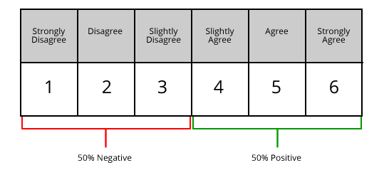
Topic 19: Scaling
Overview
What is scaling?
Five criteria for assessing scales
Likert scaling
Guttman Scaling
What is scaling?
Scaling involves rank-ordering individuals in terms of whether they possess more (or less) of the target property e.g. alienation, political interest, authoritarianism
We’re trying to assign a single representative value or score to a complex attitude or behaviour.
Ex: College student might be judged on a myriad of possible levels.
The individual’s score on the scale is determined by his or her responses to a series of questions, each of which provides some indication of the individual’s relative alienation, political interest, etc.
Combining items to form a scale serves two important functions:
- reduces measurement error and thus enhances reliability and validity. A single item may produce idiosyncratic results and/or capture only a limited aspect of the target property
- simplifies data analysis
-scale is measuring instrument, therefore must remember properties of good measures
Ex: The Cubans are evil and cannot be trusted: need to be more specific in statesments.
Five criteria for assessing scales
- unidimensionality—the scale should measure one property and one property only
- linearity and equal intervals—increasing scores should correspond to increasing amounts of the target property and the scores should be based on interchangeable units
- reliability—the scale should assign values consistently
- validity—the scale should measure the target property
- reproducibility—knowing an individual’s total score should enable us to predict correctly which items s/he agreed with and which items s/he disagreed with
Likert scaling I
Likert’s primary concern was unidimensionality.
He eliminated the need for judges (as required by Thurstone’s method) by getting respondents in a pilot sample to place themselves on an attitude continuum running from “strongly agree” to “strongly disagree” on a series of statements relating to the attitude to be measured.
Likert scaling requires a pool of attitude statements, some indicating a favourable attitude and some indicating an unfavourable attitude—but none worded so blandly that almost everyone would agree or so extremely that almost everyone would disagree.
These statements are administered to a pilot sample of 100 or more respondents who are similar to those who will be participating in the survey proper. Each respondent is asked to indicate how strongly s/he agrees or disagrees with each statement.
Each respondent’s responses are scored. Scores typically range from 1 to 5 (more complex scoring schemes have been shown to possess no advantages). The researcher has to decide whether ‘1’ indicates a very favourable attitude or a very unfavourable attitude. It does not matter as long as the scoring is consistent.
If ‘5’ indicates a very favourable attitude, strongly agreeing with a favourable statement is scored ‘5’ and so is disagreeing with an unfavourable statement.
Once the individual responses have been scored, a total score is computed for each respondent by simply adding up the scores for each statement (hence the alternative name of summated rating scale). If there are 20 statements, possible scores will range from 20 to 100.
Likert scaling III
The next step is to perform an item analysis to determine which are the best items to retain in the final scale. The purpose of this analysis is to ensure unidimensionality. There are three different ways to do this:
- correlate each statement with a reliable criterion that is known or assumed to reflect the target attitude and retain those statements that produce the highest correlations. Such external criteria are typically not available.
- internal consistency method—for each statement, correlate the score with the respondent’s total score minus the score for that statement. Retain those statements that produce the highest correlations. Factor analysis (correlate every item with every other tieam. Search for measurs that intercorrelate highly) offers a more sophisticated way of ensuring internal consistency
-Both ways of ensuring internal consistency have been criticized for violating the assumptions underlying the statistical methods employed (i.e. using ratio-level methods with ordinal-level data)
- index of item discrimination—retain those statements that best distinguish between respondents scoring in the top 25% and respondents scoring in the bottom 25%. If respondents with high scores and respondents with low scores respond similarly to a given statement, it cannot be measuring the same attitude as the statements as a whole.
-Once the statements have been selected, the scale is administered to respondents in the survey proper and their total scores are calculated. Scores are typically averaged in order to yield a scale that runs from 1 to 5 (purists use the median score since the level of measurement is only ordinal).
Advantages of Likert scales:
- reliability—respondents like the format and find it easier to answer when they can qualify their agreement or disagreement. Perform consistently
- ease of construction
- unidimensionality—if the statements are internally consistent and/or discriminate among respondents, it is likely that they are all measuring the same attitude.
Disadvantages
-lack of reproducibility—the same total score (or average score) can be obtained in many different ways. Two respondents may have the same total score and yet have answered quite differently
-unidimensionality is no guarantee of validity.
-lack of equal intervals—this criticism is questionable since it is unrealistic to think that we could come up with equal ‘units’ of alienation, interest, authoritarianism, etc.
-measuring the same thing, but not necessarily the target property
Guttman scaling I
In Guttman scaling, the twin concerns are achieving unidimensionality and reproducibility. Reproducibility means that we can predict a respondent’s responses to individual scale items knowing only his or her total score
Specifically, Guttman scaling enables us to predict each respondent’s responses to individual items with no more than 10% error for the sample as a whole.
The items that comprise a Guttman scale have the properties of being ordinal and cumulative. (can rank order in terms of having more or less of the property)
The scale is like a ladder—if someone has reached a higher rung, we can be fairly sure that they have climbed the lower rungs as well. Similarly, if the respondent says ‘yes’ to an item that indicates more of the property being measured, we can be reasonably confident that s/he will also have said ‘yes’ to all of the items that indicate less of the property.
-aim for somewhat equal intervals, avoid a big leap.
Guttman scaling II
Creating a Guttman scale involves using scalogram analysis to test a set of items for scalability. Scalogram analysis enables us to see how far our items and people’s responses to them deviate from perfect reproducibility. Scalability is indicated by a coefficient of reproducibility of .90 or higher.
It involves arranging and re-arranging both the items and the respondents in a table. The items are ordered across the top of the table from most to least according to the number of ‘yes’ responses they received. Respondents are ordered down the side of the table from most to least according to how many ‘yes’ answers they gave. Software is available for this purpose.
Guttman scaling II
The aim is to achieve a triangular pattern:
Items that produce too many deviations from these patterns are dropped and so are redundant items (i.e. items that do not lead to greater differentiation among respondents). Also dropped are items to which almost everyone said ‘yes’ (or almost everyone said ‘no’) to guard against inflated estimates of reproducibility.
If we have a large sample of respondents, we should randomly divide the sample into subsamples and repeat the scalogram analysis for each subsample to check for consistency.
Advantages of Guttman scaling:
- while there is no guarantee of unidimensionality, it is likely that items that meet the test of scalability are measuring the same property.
- reproducibility is high by definition.
- produces short but highly effective scales.
- can be used to scale behaviours and events (e.g. political participation, acts of international aggression) as well as attitudes.
Disadvantages
-may be impossible to achieve an acceptable level of reproducibility.
-items may scale in a pilot study but not in the survey proper. Not all areas of study will yield an acceptable Guttman’s scale.

Topic 20:Designing a sample
Overview
Probability versus non-probability sampling
Simple random samples
Systematic random samples
Proportionate stratified random samples
Disproportionate stratified random samples
Multi-stage random cluster samples
Convenience samples
Purposive samples
Quota samples
Probability versus non-probablity sampling
In probability (or random) sampling, every member of the population has a known and non-zero probability of being included in the sample.
In non-probability (or non-random) sampling, there is no way of specifying the probability of inclusion and there is no assurance that every member of the population has at least some probability of inclusion.
Probability sampling has two crucial advantages:
-it avoids conscious or unconscious bias on the researcher’s part because the research has no say in deciding which cases get included
-it allows us to use inferential statistics to estimate the likelihood that our sample results differ from those we would have observed if we had studied the entire population.
Despite these advantages, non-probability sampling is used when:
- the advantages of convenience and economy outweigh the risk of having an unrepresentative sample. Short notice.
- no population list or surrogate population list is available. Can only do probability if access to full population list.
Simple random samples
Simple random sampling is the most basic probability sampling design and forms the basis for more complex designs.
Simple random sampling gives every member of the population an equal probability of inclusion and gives every possible combination (of the desired sample size) of members of the population an equal probability of inclusion.
For a small population, a simple random sample can be drawn using the lottery method. For larger samples, a random number generator is used.
Disadvantages:
- can produce extreme samples (e.g. only the rich, only the poor) because every possible combination of people has an equal probability of inclusion. This is improbable, but it is not impossible.
- tedious and time-consuming unless a population list is available in an electronic format.
Systematic random samples I
Systematic random sampling involves dividing the total population size by the desired sample size to yield the sampling interval (which is conventionally denoted ‘k’). Then, beginning with a randomly selected person from among the first k people, the researcher selects every kth person. Example:
Population size = 10,000 Desired sample size = 500 k = 10,000/500 = 20
The researcher would randomly select one person from among the first 20—say, the 14th person–and then select every 20th person (14, 34, 54, 74, etc.)
Provided the first person is selected randomly, there is a priori no restriction on the probability of inclusion.
Systematic random samples II
Advantages:
- less cumbersome than simple random sampling—only one random number is required and thereafter it is simply a matter of counting off every kth
- reduces the risk of extreme samples since only combinations of people k people apart have an equal probability of inclusion.
Disadvantages
-can produce extreme samples if there is a cyclical order in the population list and this order coincides with the sampling interval.
-Only feasibly with small populations
Proportionate stratified random samples I
Proportionate stratified random sampling is used to ensure that key groups within the population are represented in the correct proportion. It provides a better solution to the problem of extreme samples.
Instead of sampling the entire population, the population is divided into homogeneous groups, or ‘strata’, and a series of samples is selected, one from each stratum. These samples are then combined to produce a representative sample of the population as a whole.
The number of people selected from each stratum is proportional to that stratum’s share of the population. Simple random sampling or systematic random sampling is used to select the samples from the strata and so there is no departure from the principle of randomness
The stratification variables must be:
- relevant to the phenomenon to be explained i.e. people within strata should be similar with respect to the DV—and people in different strata should differ with respect to the DV.
- operationalizable—this means that we require information about the value of each person in the population on the stratification variable(s) before conducting our study.
Advantages
- avoids extreme samples for the characteristics that are used to stratify the population
- increases the level of accuracy for a given total sample size OR achieves the same accuracy at a lower cost. This follows from the formula that is used to calculate the confidence interval
Stratification reduces variability (S)–and the less variability there is in the population being sampled, the smaller the error term (E) will be. Or, conversely, the less variability there is, the smaller the sample size (N) can be to achieve the same level of accuracy (E)
Disproportionate stratified random samples
Disproportionate stratified random sampling is the same as proportionate stratified random sampling except that the research deliberately over-samples some strata and/or under-samples others.
This is done for analytical reasons:
- to facilitate statistical analysis by having an equal number of cases in the different categories of the IV.
- to ensure sufficient cases for meaningful analysis where a stratum is small but substantively or theoretically important.
By definition, people belonging to some strata have a higher probability of inclusion. This is no problem when the sub-samples are being analysed separately or comparatively. However, if the sub-samples are combined into a single sample, corrective weights must be used ensure proportionality.
Multi-stage random cluster samples I
All the methods described so far require a complete list of the population. Multi-stage cluster sampling is used when no population list is available (e.g. all university students in Canada, all eligible voters, all Catholics). Sampling proceeds in stage.
At the first stage, the researcher randomly selects groupings, or ‘clusters’, of population members (e.g. a university is a ‘cluster’ of university students). At the second stage, the researcher randomly selects people from within the selected ‘clusters’. So lists only have to be obtained and/or compiled for the selected clust65ers.
Depending on the population being sampled, several stages may be involved.
e.g. randomly selecting electoral districts, then randomly selecting polling divisions within the selected districts, and finally selecting eligible voters from the selected polling divisions.
Or randomly selecting school boards, then randomly selecting schools from within the selected school boards, then randomly selecting students from within the selected schools.
Advantages
- obviates the need for a complete population list.
- reduces costs in sampling a geographically scattered population by concentrating interviews within selected localities.
Disadvantages
- increases the risk of sampling error because each stage has its associated risk of sampling error.
Accuracy can be increased by:
- increasing the sample size—but there is a trade-off between increasing the number of clusters to be selected and increasing the number of cases to be selected from those clusters.
- increasing accuracy by reducing variability—i.e. combine stratification with multistage random cluster sampling.
-so far: all avoid bias. Enable to use inferential statistics, can be simple/complex.
Convenience samples
There are three different basic non-probability sampling designs. In increasing order of desirability, they are: convenience sampling, purposive sampling and quota sampling.
Convenience sampling is just what its name implies—the researcher selects whatever people happen to be conveniently available e.g. the first 100 people who agree to be interviewed, students in an introductory psychology class.
This method is easy and inexpensive—but it is likely to yield unrepresentative samples. It should only be used (if at all) for pilot studies or for pre-testing questions.
Purposive samples
Purposive (or judgmental) sampling offers a better approach. The researcher uses his or her judgement and knowledge of the target population to select the sample, purposively trying to obtain a sample that appears to be representative.
With this method, the probability of being included depends entirely upon the judgement of the researcher.
In the hands of a skilled researcher, this method has been known to yield surprisingly accurate sample estimates.
Quota samples I
Quota sampling is the most sophisticated method of drawing a non-probability sample. The goal is to select a sample that represents a microcosm of the target population.
Interviewers are given a quota of individuals to select, specified by attributes such as age, sex, ethnicity, education, and income. They are required to select individuals displaying various combinations of these characteristics in proportion to their share of the population.
Quota sampling II
This method is generally superior to convenience or purposive sampling, but it has several limitations:
- it requires up-to-date and accurate information about the target population.
- there is ample opportunity for bias—the only constraint is that interviewers fill their quotas. The selected individuals may display the requisite combination of characteristics, but that does not guarantee their representativeness.
- the number of characteristics that can be taken into account in determining quotas is limited. Say there are four characteristics—sex plus religion (4 categories), ethnicity (3 categories), and education (4 categories). That means 2 x 4 x 3 x 4 = 96 different types of people i.e. it becomes prohibitively expensive to track down people who meet the quota requirements.

TOPIC 21 Data Gathering Techniques
Overview:
Basic Ethical Principles
The meaning of informed consent
Why can the principle of informed consent be problematic?
The cost-benefit approach
Basic Ethical Principles:
- There should be no deception involved in the research
- There should be no harm (physical, psychological or emotional) done to participants.
- Participation should be voluntary
- Participation should be based on informed consent.
The Meaning of Informed Consent:
Informed consent can be defined as ‘the procedure in which individuals choose whether to participate in an investigation after being informed of facts that would be likely to influence their decision.
This definition raises 4 issues:
– Competence – do participants have the mental or emotional capacity to provide consent?
– Voluntarism – are participants in a situation where they can exercise self-determination
– Full information – do participants have the information they need to give informed consent?
– Comprehension – do participants understand the potential risk involved?
Why can the principle of informed consent be problematic?
How much information is needed to consent to be ‘informed’?
- What if it is extremely important that participants not know the true purpose of the study?
- The trade-off between ethnical considerations and methodological considerate is often cast in terms of a conflict of rights.
Balancing Respect for Human dignity, Free and Informed Consent, Vulnerable people. Privacy and confidentiality, justice and inclusiveness, harms and benefits, minimizing harm May cause embarrassment, loss of trust in social relations, lower self-esteem. There can be cases of risk of physical harm: Rex Brynen interviews people diplomatic in bag for information.
The Cost-benefit Approach:
- The cost-benefit approach involved weighing the potential contribution to knowledge and human welfare against the potential negative effects on the dignity and welfare of the participants.
This approach can be problematic:
- The ethical issues involved can be subtle, ambiguous and debatable.
- We are not necessarily weighing predictable costs and benefits but possible costs and benefits.
- The process of balancing cost and benefits is necessarily subjective and value-laden.
Milgram’s obedience to authority: this is the ethical research. It was the research that triggered the ethical questions.
- Emotional psychological stress shapes people’s actions.
- Milgram test: if someone gave the wrong answer they were shocked at an incrementally higher rate from shock to shock.

TOPIC 22 Observational-Methods
What is observational research?
Some advantages of observational research
The trade-offs involved in observational research
Types of observational research
Other drawback of observational research.
What is Observational Research?
- It is the direct observation of political behaviour as it occurs in the natural setting. The researcher can study the behaviour as it occurs.
- Observational research differs from other methods, observational research melds data collection and theory generating. The researcher doesn’t come in with carefully formulated hypothesis.
- Data collection and data analysis are not discrete stages. Instead, the researcher attempts to develop a generalized understanding of an unfolding process over an extended time period, through a blend of induction and deduction.
Some advantages of observational research
- Flexibility – the research can modify the research design in the light of emerging theoretical understandings and/or changes in the situation being studied.
- Feasibility – no elaborate preparations necessary.
- Low cost – observational research does not require expensive equipment or staff.
- Depth of understanding – observational research enable the research to develop a comprehensive and nuanced understanding.
- External validity – behaviour is studied in its natural setting (minimizes or eliminates artificiality)
- Contextual understanding – the researcher is able to analyse the context in which behaviour occurs.
- Immediacy – the research does not have to rely on participants’ recall.
The Trade-Offs involved in observational research
Ethical considerations, reactivity and access.
- If people know they are being observed, their behaviour may be affected. They may even refuse permission. BUT if they are observed without their permission or under false pretences in order to avoid the reactivity problem and/or solve the access problem, the research becomes ethically problematic.
Types of observational research I
- Covert participant observation is intended to solve both the reactivity problem and the access problem. The researcher is either a genuine participant in what is being observed or pretend to be a genuine participant.
- The researcher’s true identity is unknown to the other participants. They perceive the researcher to be just another participant BUT:
- This type of observational study raises significant ethical issues (lack of informed consent, deception, violation of privacy).
- It does not necessarily solve the reactivity problem (the research’s own behaviour may affect the behaviour under study).
- There is a risk of getting caught up in the assumed role.
Types of observational research II
- Assuming the role of participant-as-observer is intended to resolve the ethical issue, but poses problem of reactivity.
- The researchers participates fully in the behaviour under study, but make it clear that he or she is also undertaking research.
- The difficulty with this type of research is being accepted in this role. Access may be denied.
Types of observational research III
- In the role of observer-as-participant, the researcher identifies him or herself as a researcher and makes no pretence of being a participant.
- There are still the problems of access and reactivity, but there is less risk of getting caught up in the behaviour that is being observed.
- Finally, there is the role of complete observer. The researcher observes the behaviour without becoming part of it in any way. Typically, the behaviour is being observe in a setting that is regularly open to the public.
- This role avoids ethical dilemmas and the problems of access and reactivity. The researcher is less likely to lose his or her scholarly perspective, but is also less likely to develop a full appreciation of the bahviour under study.
Other drawbacks of observational research:
- Unreliability – there are ample opportunities for random error and we cannot be sure that another research observing the same behaviour would draw the same conclusion.
- Lack of generalizability – because of the personal nature of the observations and the potential for biased ‘samples’
- Low transmissibility and replicability.
Difference btwn inferential & descriptive statistics and example of each